© Eike Mueller, University of Bath 2025. These notes are copyright of Eike Mueller, University of Bath. They are provided exclusively for educational purposes at the University and are to be downloaded or copied for your private study only. Further distribution, e.g. by upload to external repositories, is prohibited. html generated with pandoc using easy-pandoc-templates under the GPL-3.0.1 license

Motivation

What is Scientific Computing?

The goal of Scientific Computing is to efficiently simulate physical phenomena on a computer. The output of these simulations are numerical results which can be visualised and analysed to get a better understanding of the physical system under study or to inform decisions. For example, simulations of atmospheric flow can be used to produce weather forecasts and to help policymakers decide on strategies for mitigating the effects of climate change. Since the systems under study are typically very complex, this requires sophisticated algorithms, well-implemented code and significant computing power.

For these simulations to be useful, it is crucial to obtain accurate results in the shortest possible time: a forecast of tomorrow’s weather will not be very useful if it takes a week to produce it. The world’s first numerical weather forecast by Lewis Fry Richardson over 100 years ago took six weeks to produce; the six-hour forecast was also completely wrong! Things have moved on since then, and the Met Office nowadays routinely produces accurate and reliable forecasts for the next few days within about an hour.

The general process for simulating a complex physical phenomenon on a computer is illustrated schematically in Figure 1. It involves many steps, which require expertise from different disciplines.

Figure 1: Scientific Computing flowchart

Step 1: Modelling

The physical phenomenon first needs to be expressed in mathematical form. This requires domain-specific knowledge and some sort of judgement as to which processes need to be included or can be neglected. Often, this knowledge has been developed over a long time based on experiments and theoretical analysis. For example, the flow of fluids in the atmosphere can be modelled with the Navier Stokes equations, but there are several simplications that are often applied to obtain a simpler mathematical model. For example, one might neglect the viscosity of the fluid or assume that the atmosphere is in hydrostatic balance. No model is perfect, and hence this step will introduce modelling errors which need to be quantified. For example, in models of the atmosphere, the physics of cloud formation is still not fully understood and need to be approximated. Mathematical modelling is discussed in other courses and not the subject of this unit: in the following our starting point will be a mathematical description of the problem that we want to simulate.

In the following we will consider a variant of the Poisson equation, namely the following partial differential equation (PDE):

\[ -\nabla(\kappa \nabla u) + \omega u = f\qquad (1) \]

This equation, which is to be solved for the function $u$ for a given right hand side $f$, arises in many applications. In fact, the Met Office repeatedly solve a slightly more complicated form of this PDE to produce climate- and weather forecasts.

Step 2: Discretisation

In virtually all practically relevant cases the resulting mathematical model can not be solved analytically (of course, this depends on how the model is chosen. However, if it can be solved, this usually means that the model is too simplistic, i.e. it will only give inaccurate predictions). For example, the Navier Stokes equations for fluid flow are a system of time-dependent coupled nonlinear PDEs formulated on a non-trivial domain. These PDEs have no known closed form solution, and in fact the same applies for the problem in (1) in all but the simplest setups. To solve the problem on a computer, the continuous equations need to be discretised to obtain a finite set of equations that can be solved. Several methods can be used for this, and in this course we will employ the Finite Element Method which is widely used in science and industry. As we will see, this allows rewriting (1) as a linear algebra problem \[ A\boldsymbol{u} = \boldsymbol{b}\qquad (2) \] where $A$ is an $n\times n$ matrix and $\boldsymbol{u}, \boldsymbol{b}\in\mathbb{R}^n$ are vectors. Discretisation introduces additional errors. However, in contrast to modelling errors, these discretisation errors can usually be quantified and (at least in principle) they can be made arbitrarily small. The justification and analysis of the Finite Element Method is the topic of MA32066, which uses techniques from Numerical Analysis to investigate the accuracy and stability of the approach.

Step 3: Algorithm design

To solve the equations that arise from discretisation, we need to employ suitable numerical algorithms. For example, in many cases we need to assemble and solve large systems of linear equations of the form given in (2). While simple methods like Gaussian elimination can be employed for small problems, more sophisticated algorithms are required for the large problems that arise in real-life applications: reducing the discretisation errors below an acceptable threshold often requires the solution of problems with millions of unknowns, i.e. $n\sim 10^6$. The methods need to be robust, stable and efficient in the sense that their computational complexity should not grow too rapidly with the problem size $n$.

To illustrate this, assume that the computational complexity of the solution algorithm is $\mathcal{O}(n^3)$, and it takes $1\text{ns}=10^{-9}\text{s}$ to solve a problem with $n=10$ unknowns. Then the solution of a problem with $n=10^{6}$ unknowns will take 11 days. In contrast, an $\mathcal{O}(n)$ algorithm which takes $1\mu\text{s} = 10^{-6}\text{s}$ for $n=10$ could solve the problem with $n=10^{6}$ in $0.1 \text{s}$. As we will see later, Gaussian elimination is an $\mathcal{O}(n^3)$ algorithm and therefore impractical for most real-life applications.

In the following we will use different numerical methods for solving sparse systems of linear equations of the form given in (2), with the aim of achieving $\mathcal{O}(n)$ computational complexity. For optimal efficiency, these algorithms only provide an approximate solution, i.e. they introduce additional errors which need to be carefully balanced with the errors from modelling and discretisation. The same applies for many other solution algorithms in Scientific Computing which trade a small loss in accuracy for improved efficiency.

Step 4: Implementation

For the numerical algorithms to be useful they need to be implemented on a computer. This requires great care to ensure that the implementation is both efficient and correct. Since codes for real-life applications in Scientific Computing are often very complex, it is crucial that they are carefully designed and documented. The number of bugs can be minimised by thorough testing and systematic debugging. The code should also be optimised as much as possible to make optimal use of computational resources. In many cases well-established libraries need to be used for optimal performance. Knowing how to use external libraries is an important skill.

The focus of this unit is the implementation of the Finite Element method in Python. We will employ object oriented design techniques to map mathematical objects to Python classess. For optimal efficiency we will also build on the numpy and PETSc libraries for the solution of the numerical linear algebra problems of the form (2) that arise after discretisation.

Step 5: Run code

To obtain numerical results, the code needs to be run on a computer. Since real-life problems are very large, this often means running on a supercomputer, which requires adaptation of the code to run on several processing units in parallel to reduce the runtime to an acceptable level. While not the main focus of this unit, we will look at the fundamental concepts of parallelisation at the end of the semester. Modern supercomputers are now capable of performing more than $10^{18}$ floating point operations (FLOPs) per second, see the top 500 list of supercomputers for some examples.

It is important to understand the characteristics of the hardware to predict performance and to estimate how well the code exploits the capabilities of the machine. In this course, we will develop a simple, but widely used performance model for this purpose.

Since real numbers can only be represented approximately on a computer, rounding errors can potentially seriously distort the results of a simulation. This additional source of error needs to be taken into account during the algorithm design stage.

Abstractions and software design

During the process shown in Figure 1 the problem that we are trying to solve is expressed at different levels of abstraction. For example, the mathematical equations that descibe the model explicitly refer to physical variables such as pressure and temperature, while in the discretised equations we use a different formalism based on vectors and matrices. The computer code contains only for-loops that operate on indices and the machine code of the executable which is ultimately run on the supercomputer only operates on 0’s and 1’s.

The following diagram illustrates how the problem is expressed at different abstraction levels in the process: \[ \begin{aligned} \text{\textbf{physical}}\; & \text{\textbf{phenomenon}}\\ \downarrow\\ \text{mathematical}\; & \text{model}\\ \downarrow\\ \text{discretised}\; & \text{equations}\\ \downarrow\\ \text{algorithm}\; & \text{pseudocode}\\ \downarrow\\ \text{computer}\; & \text{code (Python)}\\ \downarrow\\ \text{executable}\; & \text{program}\\ \downarrow\\ \text{\textbf{numerical}}\; & \text{\textbf{result}}\\ \end{aligned} \] Crucially, information is lost when moving down this hierarchy: looking at a for-loop in the Python code will not tell use what the physical meaning of the corresponding variables is or how the are related to terms in the discretised equations. This makes it difficult to verify the correctness of the code since we are trying to analyse it at the wrong level.

This problem can be mitigated by mapping mathematical objects to computer code in a transparent way by using suitable abstractions and defining sensible interfaces: for example, when using the finite element method, we can map mathematical concepts such as basis functions directly to suitable classes in the Python code: the code explicitly encodes the mathematics which makes it much easier to understand and debug. We will employ this idea, which is used to great success by well-established Finite Element packages such as Firedrake, throughout this course.

Background: linear algebra, sparse matrices and tensors

Implementating the finite element method requires the manipulation of vectors and matrices. In the following we briefly review the implementation of fundamental linear algebra operations in the numpy library. Since many matrices that we will encounter in this course are sparse, we will discuss an efficient storage format for this class of matrices and describe its implementation in the Portable, Extensible Toolkit for Scientific Computation (PETSc) (pronounced “pet-see”). We will also introduce the concept of tensors, which generalise vectors and matrices, and which we will need during the assembly phase of the finite element method.

Linear algebra in numpy

In numpy, vectors and matrices are represented by objects of type np.ndarray. For example, the vectors $\boldsymbol{v}, \boldsymbol{b}\in\mathbb{R}^3$ and the $3\times 3$ matrix $A$ given by

\[ \boldsymbol{v} = \begin{pmatrix} 1.2 \\ 7.6 \\ 2.1 \end{pmatrix} \qquad \boldsymbol{b} = \begin{pmatrix} -7.2 \\ 0.6 \\ 1.3 \end{pmatrix} \qquad A = \begin{pmatrix} 4.3 & -1.2 & 2.8 \\ 0.7 & 7.3 & 1.1 \\ -0.4 & 0.2 & 9.7 \end{pmatrix} \]

can be created as follows:

import numpy as np

v = np.array([1.2,7.6,2.1], dtype=float)
b = np.array([-7.2, 0.6, 1.3], dtype=float)
A = np.array([[4.3, -1.2, 2.8],[0.7, 7.3, 1.1], [-0.4, 0.2, 9.7]], dtype=float)

Usually we can leave out the keyword argument dtype=float which explicitly specifies the data type. However, since without this keyword Python will infer the data type automatically, it is required in cases like z = np.array([1,2,4]) which by default will create an integer-valued array (in contrast, v = np.array([1.2,7.6,2.1]) will result in an array whose entries are of type float since Python interprets 1.2 as a real number).

Special matrices

It is possible to create special matrices such as the identity or a matrix containing only zeros:

identity_3x3 = np.eye(3)         # Creates a 3x3 identity matrix
zero_4x3 = np.zeros(shape=(4,3)) # Creates a 4x3 matrix containing only zeros

To test our code, we might also want to create matrices with random values. For example, a $4\times 2$ matrix with entries that are normally distributed with mean zero and variance one can be created like this:

rng = np.random.default_rng(seed=24618567)
random_4x2 = rng.normal(size=(4,2))

Observe that instead of using np.random.normal(size=(4,2)) we create a random number generator generator with a fixed seed first. This ensures that the results are the same in subsequent runs of the code which will simplify debugging.

Linear algebra operations for vectors and matrices

Numpy provides functionality for manipulating matrices and vectors. For example, we can compute the matrix-vector product $\boldsymbol{w} = A\boldsymbol{v}$ or the dot-product $\rho = \boldsymbol{v}\cdot \boldsymbol{b}$ by using the @ operator and the np.dot() method:

w = A @ v
rho = np.dot(v,b)

In contrast, the * operator will perform element-wise multiplication: The Python code

t = v * b

creates the three-dimensional vector $\boldsymbol{t}\in\mathbb{R}^3$ with

\[ \boldsymbol{t} = \begin{pmatrix} 1.2\cdot (-7.2) \\ 7.6 \cdot 0.6 \\ 2.1 \cdot 1.3 \end{pmatrix} = \begin{pmatrix} -8.64 \\ 4.56 \\ 2.73 \end{pmatrix}. \]

Solving linear systems

To solve the linear system $A\boldsymbol{u} = \boldsymbol{b}$ for some invertible square matrix $A$ we can use np.linalg.solve():

u = np.linalg.solve(A,b)

Usually this is more efficient than multiplying $\boldsymbol{b}$ by the inverse $A^{-1}$ of $A$:

u = np.linalg.inv(A) @ b # Don't do this!

For more information please refer to the numpy documentation, in particular the documentation of Linear Algebra routines.

Sparse matrices

Many matrices that arise in Scientific Computing contain a lot of zero entries. Examples can be found in the SuiteSparse Matrix Collection: clicking on the names of individual matrices will provide more details and show a visualisation of their structure.

Figure 21 shows the spy-plot of the $81\times 81$ matrix that is obtained from a finite element discretisation; we will discuss how this matrix is constructed in more detail later, for now we are only interested in how it can be stored and used.

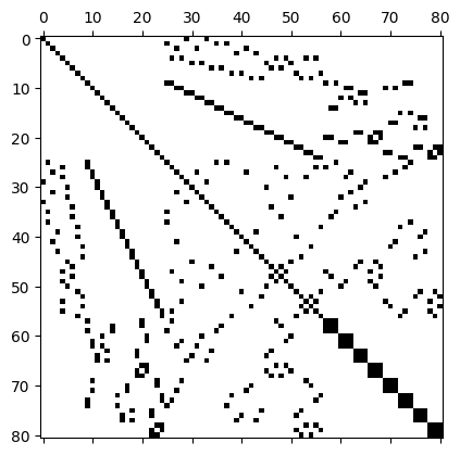
Of the $81\times 81 = 6561$ entries of this matrix, only $n_{\text{nz}}=497$ or $7.6\%$ are nonzero, which corresponds to an average number of around $\overline{n}_{\text{nz}} = 6.14$ nonzeros per row. A matrix $A$ with $n_{\text{nz}}\ll n$ nonzero entries is often called sparse. Clearly, it is very inefficient to store all these zero entries if only a fraction of entries is in fact required to encode the data stored in the matrix.

We therefore introduce a widely-used storage format which is more suitable for matrices like this.

Compressed Sparse Row storage

To store sparse matrices, we proceed as follows:

Store all non-zero entries in a long array $V$ of length $n_{\text{nz}}$, going throw the matrix row by row
For each non-zero entry also store the corresponding column index in an array $J$ of the same length as $V$

We could now also store the corresponding row-indices in an array $I$ of the same length. With this, it would then be possible to reconstruct all non-zero entries of $A$ from the three arrays $V$, $I$ and $J$:

Algorithm: Reconstruction of matrix from arrays $\boldsymbol{V}$, $\boldsymbol{J}$ and $\boldsymbol{I}$

Set $A\gets 0$
for $\ell=0,1,2,\dots,n_{\text{nz}}-1$ do
$~~~~$ Set $A_{I_\ell,J_\ell} \gets V_{\ell}$
end do

However, there is a more efficient way of doing this: Since the arrays $V$ and $J$ are constructed by going through the matrix row by row, we only need to keep track of where a new row starts. This can be encoded as follows:

Store an array $R$ of length $n+1$ such that $R_i$ describes the index in $V$, $J$ where a new row starts. For convenience, we also store $R_{n} = n_{\text{nz}}$.

The resulting storage format, consisting of the arrays $V$ (values), $J$ (column indices) and $R$ (row pointers) is known as Compressed Sparse Row storage (CSR). Given $V,J,R$ it is possible to reconstruct the matrix $A$ as follows:

Algorithm: Reconstruction of matrix in CSR format from arrays $\boldsymbol{V}$, $\boldsymbol{J}$ and $\boldsymbol{R}$

Set $A\gets 0$
Set $\ell\gets 0$
for $i=0,1,2,\dots,n-1$ do
$~~~~$ for $j=R_i,R_i+1,\dots,R_{i+1}-1$ do
$~~~~~~~~$ Set $A_{i,J_\ell} \gets V_{\ell}$
$~~~~~~~~$ Increment $\ell\gets \ell+1$
$~~~~$ end do
end do

Example

Consider the following $5\times 5$ matrix with $n_{\text{nz}}=11$ non-zero entries:

\[ \begin{pmatrix} 1.3 & 2.4 & \textcolor{lightgray}{0} & 8.7 & \textcolor{lightgray}{0} \\ 4.5 & 6.1 & \textcolor{lightgray}{0} & \textcolor{lightgray}{0} & \textcolor{lightgray}{0} \\ \textcolor{lightgray}{0} & 2.1 & 8.3 & \textcolor{lightgray}{0} & 9.4 \\ \textcolor{lightgray}{0} & \textcolor{lightgray}{0} & \textcolor{lightgray}{0} & \textcolor{lightgray}{0} & \textcolor{lightgray}{0} \\ \textcolor{lightgray}{0} & 3.7 & 1.1 & \textcolor{lightgray}{0} & 7.7 \end{pmatrix}\qquad(3) \]

We have the following arrays:

Values: $V=[1.3, 2.4, 8.7, 4.5, 6.1, 2.1, 8.3, 9.4, 3.7, 1.1, 7.7]$
Column indices: $J=[0,1,3,0,1,1,2,4,1,2,4]$
Row pointers: $R=[0,3,5,8,8,11]$

Note that one of the rows contains only zero entries.

Matrix-vector multiplication

Clearly, matrices stored in the CSR format are only useful if they can be used in linear algebra operations such as the computation of the matrix-vector product $\boldsymbol{v}=A\boldsymbol{u}$. This can be realised with the following algorithm:

Algorithm: Matrix-vector multiplication $\boldsymbol{v} = \boldsymbol{v} + A\boldsymbol{u}$ in CSR storage

Set $\ell\gets 0$
for $i=0,1,2,\dots,n-1$ do
$~~~~$ for $j=R_i,R_i+1,\dots,R_{i+1}-1$ do
$~~~~~~~~$ Set $v_i \gets v_i + V_{\ell} u_{J_{\ell}}$
$~~~~~~~~$ Increment $\ell\gets \ell+1$
$~~~~$ end do
end do

Fortunately, we do not need to implement this algorithm (and other, more complicated operations such as matrix-matrix multiplication) ourselves. Instead, we will use a suitable library.

PETSc implementation

To implement matrices in the CSR storage format, we use the Portable, Extensible Toolkit for Scientific Computation (PETSc). Since PETSc itself is written in the C-programming language, we will work with the petsc4py Python interface. After installation, this can be imported as follows:

from petsc4py import PETSc

We can now create an (empty) matrix with

A = PETSc.Mat()

To create the $5\times 5$ matrix in (3) above, we first need to set up the sparsity structure, i.e. the arrays $J$ (called col_indices) and $R$ (called row_start). This is done with the createAIJ() method, which gets passed the number of rows and columns and the keyword argument csr which is a tuple of the form $(R,J)$:

n_row = 5
n_col = 5

col_indices = [0, 1, 3, 0, 1, 1, 2, 4, 1, 2, 4]
row_start = [0, 3, 5, 8, 8, 11]

A.createAIJ((n_row, n_col), csr=(row_start, col_indices))

We can now insert values, for example we might want to set $A_{0,3} = 8.7$, as highlighted in red here: \[ \begin{pmatrix} 1.3 & 2.4 & \textcolor{lightgray}{0} & \textcolor{red}{8.7} & \textcolor{lightgray}{0} \\ 4.5 & 6.1 & \textcolor{lightgray}{0} & \textcolor{lightgray}{0} & \textcolor{lightgray}{0} \\ \textcolor{lightgray}{0} & 2.1 & 8.3 & \textcolor{lightgray}{0} & 9.4 \\ \textcolor{lightgray}{0} & \textcolor{lightgray}{0} & \textcolor{lightgray}{0} & \textcolor{lightgray}{0} & \textcolor{lightgray}{0} \\ \textcolor{lightgray}{0} & 3.7 & 1.1 & \textcolor{lightgray}{0} & 7.7 \end{pmatrix} \] This can be done by calling the setValue() method:

# Set 
row = 0
col = 3
value = 8.7
A.setValue(row, col, value)

Trying to set an element which is not part of the sparsity structure (such as row=4, col=2) will result in an error. Note that the setValue() method has an optional parameter addv. For addv=True the value will be added to an already existing value and for addv=False already existing entries will be overwritten.

We can also set blocks of several values. For example, we might want to set the $2\times 2$ block in the upper left corner, as highlighhted in red here: \[ \begin{pmatrix} \textcolor{red}{1.3} & \textcolor{red}{2.4} & \textcolor{lightgray}{0} & 8.7 & \textcolor{lightgray}{0} \\ \textcolor{red}{4.5} & \textcolor{red}{6.1} & \textcolor{lightgray}{0} & \textcolor{lightgray}{0} & \textcolor{lightgray}{0} \\ \textcolor{lightgray}{0} & 2.1 & 8.3 & \textcolor{lightgray}{0} & 9.4 \\ \textcolor{lightgray}{0} & \textcolor{lightgray}{0} & \textcolor{lightgray}{0} & \textcolor{lightgray}{0} & \textcolor{lightgray}{0} \\ \textcolor{lightgray}{0} & 3.7 & 1.1 & \textcolor{lightgray}{0} & 7.7 \end{pmatrix} \] For this, we need to specify the rows and columns in the target matrix and use the setValues() method as follows:

rows = [0, 1]
cols = [0, 1]
local_matrix = np.array([1.3, 2.4, 4.5, 6.1])
A.setValues(rows, cols, local_matrix)

Blocks do not have to be contiguous but they have to have a tensor-product index structure defined by rows $\otimes$ cols. We could, for example, to set the 6 non-zero values highlighted in red here: \[ \begin{pmatrix} 1.3 & 2.4 & \textcolor{lightgray}{0} & 8.7 & \textcolor{lightgray}{0} \\ 4.5 & 6.1 & \textcolor{lightgray}{0} & \textcolor{lightgray}{0} & \textcolor{lightgray}{0} \\ \textcolor{lightgray}{0} & \textcolor{red}{2.1} & \textcolor{red}{8.3} & \textcolor{lightgray}{0} & \textcolor{red}{9.4} \\ \textcolor{lightgray}{0} & \textcolor{lightgray}{0} & \textcolor{lightgray}{0} & \textcolor{lightgray}{0} & \textcolor{lightgray}{0} \\ \textcolor{lightgray}{0} & \textcolor{red}{3.7} & \textcolor{red}{1.1} & \textcolor{lightgray}{0} & \textcolor{red}{7.7} \end{pmatrix} \] The indices of these values are described by the tensor product $(2,4)\otimes(1,2,4)$, and hence we need to do this:

rows = [2, 4]
cols = [1, 2, 4]
A_local = np.array([2.1, 8.3, 9.4, 3.7, 1.1, 7.7])
A.setValues(rows, cols, A_local)

Finally, before we can use the matrix for any computations, we need to assemble it:

A.assemble()

For debugging purposes, we might want to print out the matrix. This can be done by first converting the sparse matrix A to a dense matrix A_dense and then extracting the numpy array A_numpy which represents the values:

A_dense = PETSc.Mat()
A.convert("dense",A_dense)
A_numpy = A_dense.getDenseArray()

Obviously, this only makes sense for relatively small matrices.

PETSc provides a lot of additional functionality for manipulating matrices, see the documentation of petsc4py.PETSc.Mat for further details.

Vectors and matrix-vector multiplication

PETSc also provides a vector class. To create vectors such as the five-dimensional $\boldsymbol{v}\in\mathbb{R}^5$ with \[ \boldsymbol{v} = \begin{pmatrix} 8.1\\0\\9.3\\-4.3\\5.2 \end{pmatrix} \] we can do this:

v = PETSc.Vec()
v.createWithArray([8.1, 0, 9.3, -4.3, 5.2])

We can now multiply the matrix that we created above with this vector to compute $\boldsymbol{w}=A\boldsymbol{v}$. For this, we first need to create an empty five-dimensional vector $\boldsymbol{w}$ to hold the result, which can be done with the createSeq() method.

w = PETSc.Vec()
n = 5
w.createSeq(n)

With this, the mult() method can be used to multiply $A$ and $\boldsymbol{v}$:

A.mult(v, w)

Instead, we can also just use the @ operator, as for numpy matrices/vectors:

w = A @ v

To print the vector we need to first extract the underlying array with the getArray() method:

w_numpy = w.getArray()
print(w_numpy)

For more information on PETSc vectors see the documentation of petsc4py.PETSc.Vec.

Tensors

Tensors are generalisations vectors and matrices: they can be understood as $d$-dimensional arrays. A tensor $T$ of rank $d$ is an object which can be indexed with $d$ integers $i_0,i_1,\dots,i_{d-1}$ where $0\le i_k < s_k$ for $k=0,1,2,\dots,d-1$, i.e. we can write $T_{i_0,i_1,\dots,i_{d-1}}\in \mathbb{R}$ for the tensor elements. The list $[s_0,s_1,\dots,s_{d-1}]$ is known as the shape of the tensor. We are already familiar with three special cases:

rank 0 tensors are scalars, i.e. real numbers $\sigma\in\mathbb{R}$. In this case the shape is the empty list $[\;]$.
rank 1 tensors are vectors $\boldsymbol{v}\in \mathbb{R}^n$ with elements $v_i$ for $0\le i< n$. The shape of a vector is the single number $[n]$, i.e. the dimension of the vector.
rank 2 tensors are $n\times m$ matrices $A\in \mathbb{R}^{n\times m}$ with elements $A_{ij}$ for $0\le i<n$ and $0\le j <m$. The shape is the tuple $[n,m]$, where $n$ is the number of rows and $m$ is the number of columns of the matrix.

Tensors in numpy

In numpy, (real-valued) tensors are represented by multidimensional arrays of type np.ndarray(...,dtype=float). For example, we can create a rank 3 tensor of shape $[2,3,4]$ with only zero entries like this:

T = np.zeros(shape=[2,3,4],dtype=float)

or construct the $2\times 3$ matrix $\begin{pmatrix}1.8 & 2.2 & 3.4 \\ 4.2 & 5.1 & 6.7\end{pmatrix}$ of shape $[2,3]$ like this:

A = np.array([[1.8,2.2,3.4],[4.2,5.1,6.7]],dtype=float)

The shapes are given by T.shape and A.shape respectively.

Adding tensors and elementwise multiplication

Tensors $T$, $T'$ of the same shape can be scaled and added elementwise: if $\alpha,\beta\in \mathbb{R}$ are real numbers, then $S=\alpha T+\beta T'$ is a new tensor of the same shape. The entries of $S$ are given by

\[ S_{i_0,i_1,\dots,i_{d-1}} = \alpha T_{i_0,i_1,\dots,i_{d-1}}+\beta T'_{i_0,i_1,\dots,i_{d-1}} \qquad \text{for all $i_0,i_1,\dots,i_{d-1}$ with $0\le i_k < s_k$ for $k=0,1,2,\dots,d-1$}. \]

In numpy this can be implemented like this:

S = alpha*T + beta*Tprime

As for vectors and matrices, tensors can be multiplied element-wise: if $T$, $T'$ are tensors of the same shape, then their elementwise product $P=T*T'$ is a new tensor of the same shape. The entries of $P$ are given by

\[ P_{i_0,i_1,\dots,i_{d-1}} = T_{i_0,i_1,\dots,i_{d-1}}T'_{i_0,i_1,\dots,i_{d-1}} \qquad \text{for all $i_0,i_1,\dots,i_{d-1}$ with $0\le i_k < s_k$ for $k=0,1,2,\dots,d-1$}. \]

In fact, Python allows the addition and elementwise multiplication of tensors of different shapes according to a set of broadcasting rules.

Multiplying tensors

Tensors can be multiplied in different ways by summing over repeated indices; this is often also called “contracting indices”. For example, we can multiply the rank 3 tensor $T$ and the rank 4 tensor $T'$ to obtain a rank 5 tensor $R$ as follows:

\[ R_{ijm\ell n} = \sum_{k} T_{ijk} T'_{mk\ell n}\qquad (4) \]

In numpy, indices can be contracted with the powerful numpy.einsum() method. For example, to compute $R$ according to (4) we can write

R = np.einsum("ijk,mkln->ijmln",T,Tprime)

Alternatively, we could also compute a rank 1 tensor $S$ from $T$, $T'$ and the rank 2 tensor $T''$:

\[ S_{\ell} = \sum_{ijk} T_{ijk} T'_{kjni} T''_{n\ell}\qquad (5) \]

To compute $S_{\ell}$ according to (5), we can use

S = np.einsum("ijk,kjni,nl->l",T,Tprime,Tprimeprime)

Note that the order of the indices matters! The matrix-vector product $\boldsymbol{v}=A\boldsymbol{w}$ is a special case:

\[ v_i = \sum_j A_{ij}w_j \]

In numpy, this can be implemented as

v = np.einsum("ij,j->i",A,w)

or alternatively simply as

v = A @ w

The latter is usually preferred since it is easier to understand what the code does.

Contractions can also result in a scalar. For example

\[ \boldsymbol{v}\cdot \boldsymbol{w} = \sum_i v_i w_i, \] is the dot-product of two vectors $\boldsymbol{v}$ and $\boldsymbol{w}$ which can be implemented as

np.einsum("ii->",v,w)

Similarly, the trace of a matrix $A$ defined by \[ \operatorname{trace}(A) = \sum_{i} A_{ii} \] can be computed with

np.einsum("ii->",A)

or alternatively with

np.trace(A)

Look at the documentation of numpy.einsum() for further details.

The Finite Element Method

In the following we will give a brief overview of the finite element method and review some of the fundamental ideas as to why it works. The details of the implementation will be discussed in later lectures and the theory is the subject of MA32066.

Model problem

In this course we will focus on the following partial differential equation (PDE) of the diffusion-reaction type in some bounded domain $\Omega\subset \mathbb{R}^2$: \[ -\nabla \cdot (\kappa \nabla u(x)) + \omega\; u(x) = f(x) \qquad \text{for $x\in \Omega$}\qquad(6) \] with boundary condition $\kappa\; n\cdot \nabla u(x)=g(x)$ for $x\in\partial \Omega$. Here $n=(n_0,n_1)^\top\in\mathbb{R}^2$ is the unit outward normal vector at a particular point on the boundary with $\|n\|_2 = \sqrt{n_0^2+n_1^2}=1$. We assume that $\omega, \kappa>0$ are positive constants and $f$, $g$ are given real-valued functions. Using zero-based indexing (as is used in Python) we will write $x=(x_0,x_1)^\top\in\mathbb{R}^2$ such that $\nabla=(\frac{\partial}{\partial x_0},\frac{\partial}{\partial x_1})^\top$ is the nabla-operator.

Note that in the case $\kappa=1$, $\omega=0$ the problem would reduce to the Poisson equation $-\Delta u(x)=f(x)$. Unfortunately, for the given boundary condition the solution of the Poisson equation is not unique (if the function $u$ is a solution then so is the function $u+C$ for an arbitrary constant $C$), which is why we do not consider this case here. However, the methods developed in this course can be readily applied to this setup, provided we extend them to handle Dirichlet boundary conditions of the form $u(x)=\widetilde{g}(x)$ for $x\in\partial \Omega$ and some given function $\widetilde{g}$.

Weak solutions

To solve (6), we seek solutions $u$ in some function space $\mathcal{V}$; we will discuss suitable choices for $\mathcal{V}$ below. In a finite element setting we usually only aim to determine the solution in the weak sense: Find $u\in \mathcal{V}$ such that \[ \int_\Omega \Big(-v(x)\nabla \cdot(\kappa \nabla u(x)) + \omega\; v(x) u(x)\Big)\;dx = \int_\Omega f(x) v(x)\;dx \qquad \text{for all $v \in \mathcal{V}$}. \] The function $v$ is often called a test function. Observe that in contrast to (6) we no longer require that the equation is satisfied at every point $x$. Discussing in which sense these weak solutions are equivalent to solutions of (6) (which is sometimes also referred to as the “strong” form of the equation) is beyond the scope of this course.

After integrating the first term under the integral on the left-hand side by parts, the weak form becomes \[ \int_\Omega \left(\kappa \nabla v(x) \cdot \nabla u(x) + \omega\; v(x) u(x)\right)\;dx - \int_{\partial \Omega } v(x)\;\kappa\;n\cdot \nabla u(x)\;ds = \int_\Omega f(x) v(x)\;dx.\qquad(7) \] Crucially, in contrast to (6), only first derivatives of the solution $u$ and test function $v$ are required now. This has the advantage that functions in $\mathcal{V}$ only need to be differentiable once. Using the boundary condition $\kappa\; n\cdot \nabla u(x)=g(x)$ for $x\in\partial\Omega$, we can rewrite the weak form (7) as \[ \int_\Omega \left(\kappa \nabla v(x) \cdot \nabla u(x) + \omega\; v(x) u(x)\right)\;dx = \int_\Omega f(x) v(x)\;dx + \int_{\partial \Omega} g(x) v(x)\;ds.\qquad(8) \] where only the left hand side depends on the unknown function $u$.

Let us define the symmetric bilinear form $a(\cdot,\cdot): \mathcal{V}\times \mathcal{V} \rightarrow \mathbb{R}$ with \[ a(u,v) := \int_\Omega \left(\kappa \nabla u(x) \cdot \nabla v(x) + \omega\; u(x) v(x)\right)\;dx\qquad(9) \] and the linear form $b(\cdot):\mathcal{V}\rightarrow \mathbb{R}$ with \[ b(v) := \int_\Omega f(x) v(x)\;dx+ \int_{\partial \Omega} g(x) v(x)\;ds. \]

Exercise

Convince yourself that $a(\cdot,\cdot)$ and $b(\cdot)$ are indeed (bi-) linear:

$a(c_1 u^{(1)} + c_2 u^{(2)},v) = c_1 a(u^{(1)},v) + c_2 a(u^{(2)},v)$ for all $c_1,c_2\in \mathbb{R}$, $u^{(1)}, u^{(2)},v \in \mathcal{V}$
$a(u,c_1 v^{(1)} + c_2 v^{(2)}) = c_1 a(u,v^{(1)}) + c_2 a(u,v^{(2)})$ for all $c_1,c_2\in \mathbb{R}$, $u,v^{(1)}, v^{(2)} \in \mathcal{V}$
$b(c_1 v^{(1)} + c_2 v^{(2)})=c_1b( v^{(1)}) + c_2 b(v^{(2)})$ for all $c_1,c_2\in \mathbb{R}$, $v^{(1)}, v^{(2)} \in \mathcal{V}$

and that $a(\cdot,\cdot)$ is symmetric:

$a(v,u) = a(u,v)$ for all $u,v\in \mathcal{V}$

With these (bi-)linear forms, we can formulate the weak problem in (8) as follows: Find $u \in \mathcal{V}$ such that \[ a(u,v) = b(v) \qquad \text{for all $v \in \mathcal{V}$}.\qquad(10) \]

Choice of function space $\mathcal{V}$

In the following we choose $\mathcal{V}:=H^1(\Omega)\subset L_2(\Omega)$, which is the space of all real-valued functions on $\Omega$ which have a square-integrable first derivative. More specifically, define the following two norms \[ \begin{aligned} \| u\|_{L_2(\Omega)} &:= \left(\int_\Omega u(x)^2\;dx\right)^{\frac{1}{2}}\\ \| u\|_{\mathcal{V}} = \| u\|_{H^1(\Omega)} &:= \left(\int_\Omega \left(u(x)^2+|\nabla u|^2\right)\;dx\right)^{\frac{1}{2}} \end{aligned} \] and then set $L_2(\Omega) = \left\{u : ||u||_{L_2(\Omega)}<\infty\right\}$ (the space of square-integrable real functions) and $H^1(\Omega) = \left\{u : ||u||_{H^1(\Omega)}<\infty\right\}$ (the space of square-integrable functions with square-integrable first derivative).

Finite element solutions

Now, obviously it is not possible to solve (10) on a computer since $\mathcal{V}$ contains infinitely many functions. Instead, we try to find solutions in a finite-dimensional subspace $\mathcal{V}_h\subset \mathcal{V}$. This could for example be the space of all functions that are piecewise linear on a given mesh with spacing $h$. We will be more precise about what that means later in this course. In this case the problem becomes: find $u_h \in \mathcal{V}_h$ such that \[ a(u_h,v_h) = b(v_h) \qquad \text{for all $v_h \in \mathcal{V}_h$ }.\qquad(11) \] Observe that this only has to hold for a finite number of test functions $v_h\in\mathcal{V}_h$.

Existence and convergence of the solution

It can be shown that (10) and (11) have unique solutions provided the linear form $b(\cdot)$ and the bilinear form $a(\cdot,\cdot)$ satisfy the following two conditions:

Boundedness: there exists some positive constant $C_+ > 0$ such that \[a(u,v) \le C_+ \|u\|_{\mathcal{V}} \|v\|_{\mathcal{V}} \qquad\text{and}\] \[b(v) \le C_+ \|v\|_{\mathcal{V}} \qquad\text{for all $u,v\in \mathcal{V}$}.\]
Coercivity: there exists some positive constant $C_- > 0$ such that \[ a(u,u) \ge C_- \|u\|_{\mathcal{V}}^2 \qquad\text{for all $u\in \mathcal{V}$}.\]

This is the famous Lax-Milgram theorem. It turns out that both conditions are satisfied for the $a(\cdot,\cdot)$, $b(\cdot)$ defined above. Furthermore, the solutions satisfy $\|u\|_{\mathcal{V}},\|u_h\|_{\mathcal{V}}\le C:=C_+/C_-$ and Cea’s Lemma states that the difference between the solution $u_h$ of (11) and the solution $u$ of (10) can be bounded as follows: \[ \|u_h - u\|_{\mathcal{V}} \le C \min_{v_h\in \mathcal{V}_h}\|u-v_h\|_{\mathcal{V}}. \] The constant $C$ on the right-hand side is problem specific since it depends on $a(\cdot,\cdot)$ and $b(\cdot)$. In contrast, the term $\min_{v_h\in \mathcal{V}_h}\|u-v_h\|_{\mathcal{V}}$ depends on the choice of function space $\mathcal{V}_h$ and describes how well the function $u \in \mathcal{V}$ can be approximated by a function $v_h\in \mathcal{V}_h$. For a suitable choice of $\mathcal{V}_h$, which we will discuss later, one can show that $\min_{v_h\in \mathcal{V}_h}\|u-v_h\|_{\mathcal{V}}\le C' h^{\mu}$ for some positive integer $\mu\ge 1$ and positive constant $C'>0$. Here $h$ is the grid-spacing of the mesh on which the problem is formulated. The constant $\mu$ depends on how well we can approximate the true solution in each grid cell. For example, if $\mathcal{V}_h$ is chosen such that functions in $\mathcal{V}_h$ can be represented by a polynomial in each grid cell, then $\mu$ will increase with the degree of this polynomial. Hence, the finite element solution $u_h$ converges to the “true” solution $u$ as the mesh is refined ($h\rightarrow 0$): \[ \|u_h - u\|_{\mathcal{V}} \le C C' h^{\mu}. \] This is why the finite element works: it can be used to systematically approximate the true solution of the PDE and the discretisation error can be made arbitrarily small by choosing a sufficiently fine mesh.

For this unit, this is all we need to know about the existence and convergence of solutions in $\mathcal{V}$ and $\mathcal{V}_h$. For further details please see the discussion in MA32066 and in [Far21] and [CH24].

Reduction to linear algebra problem

We now discuss how $u_h$ can be found in practice. Since $\mathcal{V}_h$ is finite dimensional, we can choose a basis $\{\Phi^{(h)}_k\}_{k=0}^{n-1}$ such that every function $u_h \in \mathcal{V}_h$ can be written as a linear combination of the basis functions $\Phi^{(h)}_k\in \mathcal{V}_h$: \[ u_h(x) = \sum_{k=0}^{n-1} u^{(h)}_k \Phi^{(h)}_k(x) \qquad\text{for all $x\in\Omega$.}\qquad(12) \] The vector $\boldsymbol{u}^{(h)}=(u^{(h)}_0,u^{(h)}_1,\dots,u^{(h)}_{n-1})\in\mathbb{R}^n$ is often referred to as the degrees-of-freedom vector (short: dof-vector) since its knowledge determines $u_h$. Below we will sometimes write $n_{\text{dof}}$ instead of $n$ for the total number of degrees of freedom. Picking $v_h=\Phi^{(h)}_\ell$ and inserting the expansion of $u_h$ in (12) into (11) we obtain \[ b^{(h)}_\ell:=b(\Phi^{(h)}_\ell) = a\left(\sum_{k=0}^{n-1} u^{(h)}_k \Phi^{(h)}_k,\Phi^{(h)}_\ell\right) = \sum_{k=0}^{n-1} u^{(h)}_k a\left( \Phi^{(h)}_k,\Phi^{(h)}_\ell\right), \] where we used the bi-linearity of $a(\cdot,\cdot)$. Defining the vector $\boldsymbol{b}^{(h)} := \left(b(\Phi^{(h)}_0),b(\Phi^{(h)}_1),\dots,b(\Phi^{(h)}_{n-1})\right)^\top$ and the $n\times n$ stiffness matrix $A^{(h)}$ with $A^{(h)}_{\ell k}:= a\left(\Phi^{(h)}_k,\Phi^{(h)}_\ell\right)$ we arrive at the following linear system for the dof-vector $\boldsymbol{u}^{(h)}$: \[ A^{(h)} \boldsymbol{u}^{(h)} = \boldsymbol{b}^{(h)}.\qquad(13) \]

Although $\boldsymbol{u}^{(h)}$ and $\boldsymbol{b}^{(h)}$ are both vectors in $\mathbb{R}^n$, they are constructed in a fundamentally different way:

The dof-vector $\boldsymbol{u}^{(h)}$ is a so-called primal vector: its components $u_\ell^{(h)}$ are the expansion coefficients of the function $u_h$ in (12).
In contrast, the right-hand-side vector $\boldsymbol{b}^{(h)}$ is a so-called dual vector: its components $b_\ell^{(h)}=b(\Phi_\ell^{(h)})$ are obtained by evaluating the linear functional $b(\cdot)$ for the basis functions.

The reason for this is that $b(\cdot)$ is an element of the dual space $\mathcal{V}^*$, which consists of all linear functionals defined on the space $\mathcal{V}$. We will discuss dual spaces in more detail below.

Solution procedure

In summary, the solution procedure for (11) is this:

Assemble the matrix $A^{(h)}$.
Assemble the right-hand-side vector $\boldsymbol{b}^{(h)}$.
Solve the linear system $A^{(h)} \boldsymbol{u}^{(h)} = \boldsymbol{b}^{(h)}$ in (13) for $\boldsymbol{u}^{(h)}$.
Reconstruct the solution $u_h$ from the dof-vector $\boldsymbol{u}^{(h)}$ according to the expansion in (12).

In the rest of this course we will discuss how each of these steps can be implemented in Python. The focus will be on structuring the code such that the mathematical objects are mapped to the corresponding Python objects in the source code. For the solution of the linear algebra problem in (13) we will use the PETSc library.

Finite Elements

We start by considering the weak form of the PDE for a special case, namely a domain $\Omega$ consisting of a single triangle. By doing this, we will develop the fundamental concepts and techniques of finite element analysis and discuss their implementation in Python. As we will see later, the solution of the PDE on more complicated domains can be reduced to this case.

Reference triangle

Let us consider a very simple domain $\widehat{K}=\Omega$ which consists of the right-angled triangle with vertices $\textcolor{red}{v_0=(0,0)}$, $\textcolor{red}{v_1=(1,0)}$ and $\textcolor{red}{v_2=(0,1)}$, shown in red in Figure 3. We label the edges (or facets), shown in blue, in a counter-clockwise fashion as $\textcolor{blue}{F_0 = \overrightarrow{v_1v_2}}$, $\textcolor{blue}{F_1 = \overrightarrow{v_2v_0}}$ and $\textcolor{blue}{F_2 = \overrightarrow{v_0v_1}}$. This ordering and the orientation of the edges will be important later.

In the following we will also refer to this domain as the reference triangle $\widehat{K}$.

Recall that the finite element approach starts with the choice of a suitable function space $\mathcal{V}_h$. For this, consider the space of bi-variate polynomials of degree $p$ on $\widehat{K}$:

\[ \mathcal{V}_h := \mathcal{P}_p(\widehat{K}) = \{q:q(x) = \sum_{\substack{s_0,s_1\\s_0+s_1\le p}} a_{s_0,s_1} x_0^{s_0}x_1^{s_1}\;\text{for all $x\in \widehat{K}$ with $a_{s_0,s_1}\in\mathbb{R}$}\}\subset H^1(\widehat{K}) \]

The space $\mathcal{P}_p(\widehat{K})$ is spanned by $n_{\text{dof}}=\nu = {p+2 \choose 2} = \frac{1}{2}(p+2)(p+1)$ basis functions $\{\phi_\ell\}_{\ell=0}^{\nu-1}$. These can be chosen to be the monomials $\{1,x_0,x_1,x_0^2,x_0x_1,x_1^2,\dots$}, but a better choice is to pick Lagrange polynomials. Recall that in one dimension a Lagrange interpolating polynomial is the unique polynomial of degree $m$ which passes through $m+1$ points $\{(t_k,z_k)\}_{k=0}^{m}$, i.e. $p(t_k)=z_k$ for all $k=0,1,\dots,m$. This will later allow us to construct $H^1(\Omega)$ functions on a mesh for a more general domain $\Omega$ that consists of little triangles by “glueing together” the functions on neighbouring triangles. To construct Lagrange polynomials in two dimensions, we choose $\nu$ points $\{\xi^{(\ell)}\}_{\ell=0}^{\nu-1}$ in $\widehat{K}$ and define $\phi_\ell(x)\in\mathcal{P}_p(K)$ such that \[ \phi_\ell(\xi^{(k)}) = \delta_{\ell k} = \begin{cases} 1 & \text{for $\ell=k$}\\ 0 & \text{otherwise}. \end{cases} \] A possible choice of points is given by (see Figure 4 below for some examples) \[ \{\xi^{(\ell)}\}_{\ell=0}^{\nu-1} = \left\{\left(\frac{\ell_0}{p},\frac{\ell_1}{p}\right) \quad \text{for $\ell_0,\ell_1\in\mathbb{N}$ with $0\le \ell_0\le \ell_1 \le p$}\right\}.\qquad(14) \]

We order these points (and the associated basis functions $\phi_\ell$) as follows:

Points associated with the three vertices $v_0$, $v_1$, $v_2$ (in this order); there is $\nu_{\text{vertex}}=1$ point per vertex,
points associated with the facets $F_0$, $F_1$, $F_2$ (in this order); there are $\nu_{\text{facet}}=p-1$ points per facet and on each facet these points are ordered according to the arrows in Figure 3 and finally
points associated with the interior $K^0$ of the cell $\widehat{K}$; there are $\nu_{\text{interior}}=\frac{1}{2}(p-1)(p-2)$ points of this type.

This is illustrated in Figure 4, which shows the ordering of the points for $p=1,2,3,4$:

The associated finite elements are known as Lagrange elements.

Examples

Linear finite element

For $p=1$ we obtain the (bi-)linear finite element with the following basis three functions, each of which is associated with a vertex: \[ \begin{aligned} \phi_0(x) &= 1-x_0-y_0\\ \phi_1(x) &= x_0\\ \phi_2(x) &= x_1 \end{aligned} \]

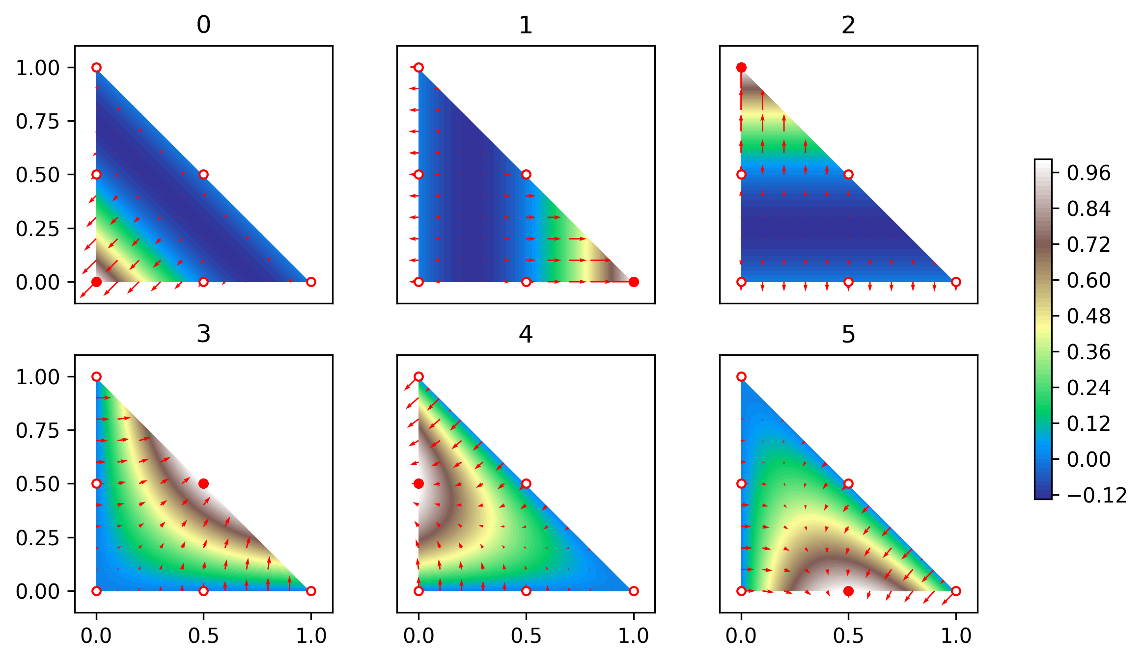
Quadratic finite element

For $p=2$ there are six basis functions, three associated with vertices \[ \begin{aligned} \phi_0(x) &= (1-x_0-x_1)(1-2x_0-2x_1),\\ \phi_1(x) &= x_0(2x_0-1),\\ \phi_2(x) &= x_1(2x_1-1), \end{aligned} \] and three associated with facets \[ \begin{aligned} \phi_3(x) &= 4x_0x_1,\\ \phi_4(x) &= 4x_1(1-x_0-x_1),\\ \phi_5(x) &= 4x_0(1-x_0-x_1), \end{aligned} \] see Figure 4. These functions are visualised in the following figure:

Formal definition of finite elements

It turns out that it is advantageous to define finite elements in a more general sense. Mirroring this more abstract mathematical definition in the Python code will help us to structure the code in a sensible way that will allow its easy adaptation to specific cases. For this we first need to introduce the notion of the dual $\mathcal{V}^*$ of a given function space $\mathcal{V}$.

Dual spaces

Consider a domain $\Omega$ and the space $\mathcal{V}=\mathcal{V}(\Omega)$ of real-valued functions $w:\Omega\rightarrow \mathbb{R}$ on $\Omega$. A linear functional $\lambda$ maps a function $w\in \mathcal{V}$ to a real value $\lambda(w)\in\mathbb{R}$ such that

\[ \lambda(c_1 w^{(1)}+c_2 w^{(2)}) = c_1\lambda(w^{(1)})+c_2 \lambda(w^{(2)}) \qquad\text{for all $c_1,c_2\in\mathbb{R}$, $w^{(1)}, w^{(2)} \in \mathcal{V}$}.\qquad(15) \]

The space of all linear functionals on $\mathcal{V}$ is called the dual space $\mathcal{V}^*$. If $\mathcal{V}$ is finite-dimensional then so is $\mathcal{V}^*$ and both spaces have the same dimension.

Examples

Let $\Omega\subset \mathbb{R}^2$ and $\mathcal{V}=H^1(\Omega)$ be the space of functions on $\Omega$ with a square integrable first derivative. Then the following $\lambda\in\mathcal{V}^*$ are linear functionals:

point evaluation: $\lambda(w) := w(\xi)$ for some point $\xi\in \Omega$
differentiation: $\lambda(w) := \frac{\partial w}{\partial x_0}(\xi)$ for some point $\xi\in \Omega$
integration: $\lambda(w) := \int_\Omega f(x)w(x)\;dx$ for some function $f \in L_2(\Omega)$

Exercise

Convince yourself that these $\lambda$ indeed satisfy (15).

Ciarlet’s definition of the finite element

This now leads to the following definition, originally due to Ciarlet (“Numerical Analysis of the Finite Element Method.” Les Presses de l’Universite de Montreal, 1976; see [Log11] for the version used here): a finite element is a triple $(\widehat{K},\widehat{\mathcal{V}},\mathcal{L})$ which consists of

the domain $\widehat{K}$ (which we will always choose to be the reference triangle in this course),
a function space $\widehat{\mathcal{V}}=\widehat{\mathcal{V}}(\widehat{K})$ of real-valued functions on $\widehat{K}$,
the degrees of freedom (or nodes) $\mathcal{L} = \{\lambda_\ell\}_{\ell=0}^{\nu-1}$ which is a basis for $\widehat{\mathcal{V}}^*$, the dual of $\widehat{\mathcal{V}}$.

Crucially, we define the finite element by choosing a basis of the dual space $\widehat{\mathcal{V}}^*$. However, we can always construct a so-called nodal basis $\{\phi_\ell\}_{\ell=0}^{\nu-1}$ of $\widehat{\mathcal{V}}$ by requiring that \[ \lambda_\ell (\phi_k) = \delta_{\ell k} \qquad\text{for all $\ell,k=0,1,\dots,\nu-1$}.\qquad(16) \]

Examples

The polynomial Lagrange element we described above is a special case of this with

$\widehat{K}$ the reference triangle
$\widehat{\mathcal{V}} = \mathcal{P}_p(\widehat{K})$, the space of bi-variate polynomials of degree $p$
$\mathcal{L}=\{\lambda_\ell\}_{\ell=0}^{\nu-1}$ with $\lambda_\ell(w) = w(\xi^{(\ell)})$ the point evaluation at the nodal points $\xi^{(\ell)}$ given in (14)

An alternative choice for the degrees of freedom would have been to define for some point $\mathring{\xi}\in \widehat{K}$: \[ \lambda_\ell (w) = \frac{\partial^{\ell_a}w}{\partial x_0^{\ell_b} \partial x_1^{\ell_a-\ell_b}}(\mathring{\xi}) \qquad\text{for $0\le \ell_b \le \ell_a\le p$ and $\ell=\frac{1}{2}\ell_a(\ell_a-1) + \ell_b$} \]

The two-dimensional Argyris finite element ([Arg68]; see Section 3.7.1 in [Log11]) is given by

$\widehat{K}$ the reference triangle
$\widehat{\mathcal{V}} = \mathcal{P}_5(\widehat{K})$, the space of quintic bi-variate polynomials
the 21 nodes (with $\nu_{\text{vertex}}=6$, $\nu_{\text{facet}}=1$, $\nu_{\text{interior}}=0$) defined as follows:
- $\lambda_\rho(w) = w(v_\rho)$ (evaluation at each vertex $v_\rho$ $\Rightarrow$ 3 nodes)
- $\lambda_{3+2\rho+a}(w) = \frac{\partial w}{\partial x_a}(v_\rho)$ (two gradient evaluations at each vertex $v_\rho$ $\Rightarrow$ 6 nodes)
- $\lambda_{9+3\rho+2a+b}(w) = \frac{\partial^2 w}{\partial x_a \partial x_b}(v_\rho)$ with $0\le a\le b\le 1$ (Hessian evaluation at each vertex $v_\rho$ $\Rightarrow$ 9 nodes)
- $\lambda_{18+\rho}(w) = n_\rho\cdot \nabla w(m_\rho)$ (normal derivative evaluation at the midpoints $m_\rho$ of each facet $F_\rho$ $\Rightarrow$ 3 nodes)

Note that the Argyris element and the quintic Lagrange element only differ in the choice of nodes. It turns out that the Argyris allows the construction of function spaces that have a bounded second derivative. We will not use the Argyris element in this course, and it is included here as an example of a finite element with non-trivial nodes.

Node numbering

As we will see later, it is crucial to establish a consistent ordering of the degrees of freedom, and here we use the same ordering as in [CH24]. For this, assume that each node is associated with a topological entity of the reference triangle $\widehat{K}$ in Figure 3. These entities are

the vertices $v_0$, $v_1$, $v_2$ in this order
the facets $F_0$, $F_1$, $F_2$ in this order
the interior $K^0$ of $\widehat{K}$

We further assume that $0\le \nu_{\text{vertex}}$ nodes are associated with each vertex, $0\le \nu_{\text{facet}}$ nodes are associated with each facet and $0\le \nu_{\text{interior}}$ nodes are associated with the interior $K^0$. Then obviously \[ \nu = 3( \nu_{\text{vertex}}+\nu_{\text{facet}})+\nu_{\text{interior}}. \] Let $\lambda_j^{(E_\rho)}$ be the $j$-th node associated with topological entity $E_\rho\in \{v_0,v_1,v_2,F_0,F_1,F_2,K^0\}$. Then we arrange the degrees of freedom $\{\lambda_0,\dots,\lambda_{\nu-1}\}$ in the order

\[ \underbrace{v_0 \rightarrow v_1 \rightarrow v_2}_{\text{(vertices)}} \rightarrow \underbrace{F_0 \rightarrow F_1 \rightarrow F_2}_{\text{(facets)}} \rightarrow \underbrace{K^0}_{\text{(interior)}} \]

i.e.

$\{\lambda_0^{(v_0)},\dots,\lambda_{\nu_{\text{vertex}}-1}^{(v_0)}, \lambda_0^{(v_1)},\dots,\lambda_{\nu_{\text{vertex}}-1}^{(v_1)}, \lambda_0^{(v_2)},\dots,\lambda_{\nu_{\text{vertex}}-1}^{(v_2)}, \lambda_0^{(F_0)},\dots,\lambda_{\nu_{\text{facet}}-1}^{(F_0)}, \lambda_0^{(F_1)},\dots,\lambda_{\nu_{\text{facet}}-1}^{(F_1)}, \lambda_0^{(F_2)},\dots,\lambda_{\nu_{\text{facet}}-1}^{(F_2)}, \lambda_0^{(K^0)},\dots,\lambda_{\nu_{\text{interior}}-1}^{(K^0)} \}$

In other words, we define the indirection map $\mu_{\text{dof}}$ such that $\lambda_{\ell=\mu_{\text{dof}}(E,\rho,j)} = \lambda_j^{(E_\rho)}$ with

\[ \mu_{\text{dof}}(E,\rho,j) = \begin{cases} \rho\cdot \nu_{\text{vertex}} + j & \text{if $E_\rho$ is the $\rho$-th vertex}\\ 3\nu_{\text{vertex}} + \rho\cdot \nu_{\text{facet}} + j & \text{if $E_\rho$ is the $\rho$-th facet}\\ 3(\nu_{\text{vertex}} + \nu_{\text{facet}}) + j & \text{if $E$ is the interior} \end{cases} \]

The inputs of the indirection map $\mu_{\text{dof}}$ are

The entity type $E$ (vertex, facet or interior)
The index $\rho$ of the particular entity; this is ignored if $E$ is the interior
The index $j$ of the unknown on the entity

This is illustrated for the polynomial Lagrange element in Figure 4. For example, for the quartic Lagrange element ($p=4$) we have that

\[ \begin{aligned} \mu_{\text{dof}}(v,1,0) &= 1\\ \mu_{\text{dof}}(F,0,2) &= 5\\ \mu_{\text{dof}}(K^0,0,2) &= 14 \end{aligned} \]

Vandermonde matrix

Having picked the nodes, how can we construct the nodal basis functions $\{\phi_\ell(x)\}_{\ell=0}^{\nu-1}$ for a given set of nodes $\{\lambda_\ell\}_{\ell=0}^{\nu-1}$? Here we follow the same procedure as in [CH24], using slightly different notation. For this, assume that we know some set of basis functions $\{\theta_m(x)\}_{m=0}^{\nu-1}$ of $\widehat{\mathcal{V}}$. For the Lagrange elements, these could for example be the monomials $1,x_0,x_1,x_0^2,x_0x_1,x_1^2,\dots$. Since $\{\theta_m(x)\}_{m=0}^{\nu-1}$ is a basis of $\widehat{\mathcal{V}}$, we can write for each $k=0,1,\dots,\nu-1$

\[ \phi_k(x) = \sum_{m=0}^{\nu-1} c_m^{(k)} \theta_m(x) \]

for some coefficients $c_m^{(k)}$. Further, since per definition $\{\phi_\ell\}_{\ell=0}^{\nu-1}$ is a nodal basis of $\widehat{\mathcal{V}}$ and $\lambda_\ell$ are linear functionals we know that

\[ \delta_{\ell k} = \lambda_\ell(\phi_k) = \sum_{m=0}^{\nu-1} \underbrace{c_m^{(k)}}_{C_{mk}} \underbrace{\lambda_\ell(\theta_m)}_{V_{\ell m}}.\qquad(17) \]

If we define the $\nu\times\nu$ matrices $V$, $C$ with $V_{\ell m} := \lambda_\ell(\theta_m)$ and $C_{mk}:=c_m^{(k)}$, then equation (17) can be written in matrix form as \[ VC = \mathbb{I}\quad \Leftrightarrow \quad C = V^{-1} \] with $\mathbb{I}$ the $\nu\times\nu$ identity matrix. In other words, we can obtain the coefficients $c_m^{(k)}$ by inverting the matrix $V$. For the Lagrange element, where $\lambda_\ell(w) = w(\xi^{(\ell)})$ are nodal evaluations and thus $V_{\ell m} = \lambda_{\ell}(\theta_m) = \theta_m(\xi^{(\ell)})$, the matrix $V$ is the Vandermonde matrix: \[ V = V(\{\xi^{(\ell)}\}_{\ell=0}^{\nu-1}) = \begin{pmatrix} 1 & \xi^{(0)}_0 & \xi^{(0)}_1 & (\xi^{(0)}_0)^2 & \xi^{(0)}_0 \xi^{(0)}_1 & (\xi^{(0)}_1)^2 & \dots \\[1ex] 1 & \xi^{(1)}_0 & \xi^{(1)}_1 & (\xi^{(1)}_0)^2 & \xi^{(1)}_0 \xi^{(1)}_1 & (\xi^{(1)}_1)^2 & \dots \\[1ex] 1 & \xi^{(2)}_0 & \xi^{(2)}_1 & (\xi^{(2)}_0)^2 & \xi^{(2)}_0 \xi^{(2)}_1 & (\xi^{(2)}_1)^2 & \dots \\[1ex] \vdots & \vdots & \vdots & \vdots & \vdots & \vdots & \ddots\\ 1 & \xi^{(\nu-1)}_0 & \xi^{(\nu-1)}_1 & (\xi^{(\nu-1)}_0)^2 & \xi^{(\nu-1)}_0 \xi^{(\nu-1)}_1 & (\xi^{(\nu-1)}_1)^2 & \dots \end{pmatrix}.\qquad(18) \] In fact, for any given set of $n$ points $\boldsymbol{\zeta}:=\{\zeta^{(r)}\}_{r=0}^{n-1}$, which do not have to coincide with the nodal points $\{\xi^{(\ell)}\}_{\ell=0}^{\nu-1}$, we can construct the $n\times\nu$ matrix $V(\boldsymbol{\zeta})$ with $V_{rm}(\boldsymbol{\zeta}) = \theta_m(\zeta^{(r)})$ in the same way. We further define the rank 3 tensor $V^{\partial}(\boldsymbol{\zeta})$ with

\[ V^{\partial}_{rma}(\boldsymbol{\zeta}):=\frac{\partial \theta_m}{\partial x_a}(\zeta^{(r)}). \]

It should be stressed that $V$ and $V^{\partial}$ can be constructed for arbitrary finite elements, not just for Lagrange elements.

Tabulation of basis functions

As we will see below, assembly of the matrix $A^{(h)}$ and right hand side vector $\boldsymbol{b}^{(h)}$ will require the evaluation (or tabulation) of the basis functions and their derivatives at a given set of points. The results from the previous section allow us to tabulate the basis functions: for a given set of points $\boldsymbol{\zeta}:=\{\zeta^{(r)}\}_{r=0}^{n-1}$, we have that

\[ T_{r\ell}(\boldsymbol{\zeta}) := \phi_\ell(\zeta^{(r)}) = \sum_{m=0}^{\nu-1} c_m^{(\ell)} \theta_m(\zeta^{(r)}) = \sum_{m=0}^{\nu-1}V_{rm}(\boldsymbol{\zeta})C_{m\ell}\qquad(19) \]

or, more compactly:

\[ T(\boldsymbol{\zeta}) = V(\boldsymbol{\zeta}) C \]

where $C=V^{-1}$ is obtained by inverting the matrix $V$ in (18).

Furthermore, we have for the derivatives

\[ \begin{aligned} T^\partial_{r\ell a}(\boldsymbol{\zeta}) &:= \frac{\partial \phi_\ell}{\partial x_a}(\zeta^{(r)}) = \sum_{m=0}^{\nu-1} c_m^{(\ell)} \frac{\partial \theta_m}{\partial x_a}(\zeta^{(r)}) \\ &= \sum_{m=0}^{\nu-1} V^\partial_{rma}(\boldsymbol{\zeta})C_{m\ell}. \end{aligned}\qquad(20) \]

Implementation

Abstract base class

Since all finite elements share the common functionality that is encapsulated in Ciarlet’s definition, we start by writing down an abstract base class FiniteElement in in fem/finiteelement.py, which establishes an interface that all concrete implementations of a finite element need to satisfy. The advantage of this approach is that we do not have to duplicate code that can be shared between all finite element implementation. Furthermore, any code that later uses a concrete finite element implementation will “know” which functionality it is allowed to use.

More specifically, each finite element should provide the following functionality:

Return the number of nodes associated with each topological entity. For this, we define abstract properties ndof_per_vertex, ndof_per_facet and ndof_per_interior for $\nu_{\text{vertex}}$, $\nu_{\text{facet}}$ and $\nu_{\text{interior}}$ respectively. The base class also contains a property ndof which returns $\nu =3(\nu_{\text{vertex}}+\nu_{\text{facet}})+\nu_{\text{interior}}$.
Tabulate the evaluation of all dofs for a given function $\hat{f}$, i.e. compute the vector $(\lambda_0(\hat{f}),\lambda_1(\hat{f}),\dots,\lambda_{\nu-1}(\hat{f}))^\top\in\mathbb{R}^\nu$. This is done with the abstract method tabulate_dofs(fhat) which gets passed a Python function fhat.
Tabulate the basis functions for a given set of points $\boldsymbol{\zeta}=\{\zeta^{(r)}\}_{r=0}^{n-1}$ which are stored as a $n\times 2$ array. This computes the $n\times\nu$ matrix $T$ with $T_{r\ell}=\phi_\ell(\zeta^{(r)})$ with the abstract method tabulate(zeta). If only a single point $\zeta\in\mathbb{R}^2$ is passed to the subroutine it should return a vector of length $\nu$.
Tabulate the gradients of all basis functions for a given set of points $\boldsymbol{\zeta}=\{\zeta^{(r)}\}_{r=0}^{n-1}$ which are stored as a $n\times 2$ array. This computes the rank 3 tensor $T^\partial$ of shape $n\times\nu\times 2$ with $T^\partial_{r\ell a}=\frac{\partial\phi_\ell}{\partial x_a}(\zeta^{(r)})$. This is done with the abstract method tabulate_gradient(zeta). If only a single point $\zeta\in\mathbb{R}^2$ is passed to the subroutine it should return a matrix of shape $\nu\times 2$.
Implement the element dof-map $\mu_{\text{dof}}(E,\rho,j)$ and its inverse. This is done with the method dofmap(entity_type,rho,j) and its inverse inverse_dofmap(ell). Since these methods will be called frequently with the same arguments, a @functools.cache decorator is added to automatically remember previously computed values.

It is crucial to observe that we carefully avoided including specific functionality (such as assuming that the basis functions are Lagrange polynomials and the degrees of freedom are point-evaluations): the base class is consistent with Ciarlet’s abstract definition of the finite element and the code mirrors the mathematical structure.

Concrete implementations

Any concrete implementations of finite elements are obtained by subclassing the FiniteElement base class. These classes have to provide concrete implementations of the following methods/properties:

ndof_per_vertex, ndof_per_facet and ndof_per_interior
tabulate_dofs(fhat) to evaluate the degrees of freedom for a given function
tabulate(zeta) to tabulate the values of the basis functions at a given set of points
tabulate_gradient(zeta) to tabulate the gradients of the basis functions for a given set of points

The finiteelements library provides the following implementations:

The bi-linear element is implemented as the class LinearElement in fem/linearelement.py
The general polynomial element is implemented as the class PolynomialElement in fem/polynomialelement.py (this class will be made available later in the semester)

If the finiteelements library has been installed, these elements can be imported as follows:

from fem.linearelement import LinearElement
from fem.polynomialelement import PolynomialElement

Numerical quadrature

The weak form of the PDE is defined via suitable integrals such as $\int_\Omega v(x)f(x)\;dx$. In general, it is not possible to evaluate these integrals exactly. Furthermore, since the finite element discretisation (replacing $\mathcal{V}\mapsto \mathcal{V}_h$ and solving the associated linear algebra problem) already introduces an error, exact integration is not necessary, provided we can find an approximate integration method with errors that are of the same order of magnitude as the discretisation.

Gauss-Legendre quadrature in one dimension

Numerical quadrature aims to approximate the integral of a function $f$ with a finite sum:

\[ \int_{-1}^{+1} f(z)\;dz \approx \sum_{q=0}^{n_q-1} \widetilde{w}_q f(\widetilde{\zeta}^{(q)}) \]

A particular quadrature rule $\mathcal{Q}=\{(\widetilde{\zeta}^{(q)},\widetilde{w}_q)\}_{q=0}^{n_q-1}$ is defined by the sets of points $\widetilde{\zeta}^{(q)}$ and corresponding weights $\widetilde{w}_q$. Here we will consider Gauss-Legendre quadrature $\mathcal{Q}^{(\text{GL})}_{n_q}$, for which the points are the roots of the Legendre polynomial $P_{n_q}$ and the weights are given by $\widetilde{w}_q = \frac{2}{(1-(\widetilde{\zeta}^{(q)})^2)(P_{n_q}'(\widetilde{\zeta}^{(q)}))^2}$. The points and weights can be constructed with numpy.polynomial.legendre.leggauss:

points, weights = numpy.polynomial.legendre.leggauss(n_q)

The details of this construction are irrelevant for this course, but we need to have some understanding of how well the numerical scheme approximates the true value of the integral. Naturally one would expect that the quadrature approximates the integral better for larger numbers of points $n_q$. Crucially, Gauss-Legendre quadrature is exact if the function to be integrated is a polynomial of degree $2n_q-1$:

\[ \int_{-1}^{+1} p(z)\;dz = \sum_{q=0}^{n_q-1} \widetilde{w}_q p(\widetilde{\zeta}^{(q)})\qquad\text{for $p\in\mathcal{P}_{2n_q-1}$} \]

We also call the degree of the highest polynomial that can be integrated exactly with a given quadrature rule the degree of precision or short “dop”: \[ \text{dop}(\mathcal{Q}^{(\text{GL})}_{n_q}) = 2n_q-1 \]

The first three Gauss-Legendre quadrature rules are shown in the following table:

number of points $n_q$	quadrature points $\widetilde{\zeta}^{(q)}$	weights $\widetilde{w}_q$	degree of precision $\text{dop}(\mathcal{Q}^{(\text{GL})}_{n_q})$
1	$0$	$2$	$1$
2	$-\frac{1}{\sqrt{3}}, +\frac{1}{\sqrt{3}}$	$1$	$3$
3	$-\sqrt{\frac{3}{5}},0,+\sqrt{\frac{3}{5}}$	$\frac{5}{9},\frac{8}{9},\frac{5}{9}$	$5$

The cases $n_q=1$ and $n_q=2$ were derived in your Numerical Analysis lecture.

While so far we have only considered integration over the interval $[-1,+1]$, it turns out that integration over more general domains and higher-dimensional can be reduced to this case.

Integration along a line

Next, imagine that we want to integrate a function along a straight line $\mathcal{C}\subset \mathbb{R}^2$ connecting two points $a,b\in \mathbb{R}^2$. To achieve this, pick a parametrisation $\gamma: [-1,1] \rightarrow \mathbb{R}^2$ of this line with $\gamma(-1)=a$, $\gamma(1)=b$

\[ \gamma(z) = \frac{1-z}{2}a+\frac{1+z}{2}b \]

then

\[ \int_{\mathcal{C}} f(x)\;ds = \frac{\|b-a\|}{2} \int_{-1}^{+1} f(\gamma(z))\;dz \] where $\|\cdot\|$ is the Euclidean norm with $\|x\| = \sqrt{x_0^2+x_1^2}$ for $x\in\mathbb{R}^2$.

Let $\mathcal{Q}_{n_q}^{(\text{GL})}=\{(\widetilde{\zeta}^{(q)},\widetilde{w}_q)\}_{q=0}^{n_q-1}$ be the Gauss-Legendre quadrature rule for the interval $[-1,+1]$. Then we obtain

\[ \int_{\mathcal{C}} f(x)\;ds \approx \sum_{q=0}^{n_q-1} w_{\mathcal{C},q} f(\zeta_{\mathcal{C}}^{(q)}) \]

where the Gauss-Legendre quadrature rule on $\mathcal{C}$ is given by $\mathcal{Q}^{(\text{GL},\mathcal{C})}_{n_q}=\{(\zeta^{(q)}_{\mathcal{C}},w_{\mathcal{C},q})\}_{q=0}^{n_q-1}$ with

\[ \zeta_{\mathcal{C}}^{(q)} = \gamma(\widetilde{\zeta}^{(q)}) = \frac{1}{2}(1-\widetilde{\zeta}^{(q)})a + \frac{1}{2}(1+\widetilde{\zeta}^{(q)})b,\qquad w_{\mathcal{C},q} = \|\gamma'(\zeta^{(q)})\| \widetilde{w}_{q} = \frac{\|b-a\|}{2} \widetilde{w}_q \] and \[ \text{dop}(\mathcal{Q}^{(\text{GL},\mathcal{C})}_{n_q}) = \text{dop}(\mathcal{Q}^{(\text{GL})}_{n_q}) = 2n_q-1. \]

Two-dimensional quadrature for the reference triangle

To numerically integrate functions over the reference triangle $\widehat{K}$ we use the same approach as in [CH24]. For this, first observe that $\widehat{K}$ is the image of the square $S=[-1,+1]\times [-1,+1]$ under the Duffy transform $\tau$ which maps a point $\widetilde{x}=(\widetilde{x}_0,\widetilde{x}_1)\in S$ to

\[ \begin{aligned} \tau(\widetilde{x}) = \begin{pmatrix}\frac{1}{2}(1+\widetilde{x}_0)\\[1ex]\frac{1}{4}(1-\widetilde{x}_0)(1+\widetilde{x}_1)\end{pmatrix} \in \widehat{K}\qquad(21) \end{aligned} \]

(see Figure 6)

Integration over $\boldsymbol{S}$

Since $S=[-1,+1]\times[-1,+1]$ is the product of two intervals, we can integrate functions over $S$ by picking quadrature points and weights $\mathcal{Q}_{n_q}^{(\text{GL},S)}=\{(\widetilde{\zeta}^{(q)},\widetilde{w}_q)\}_{q=0}^{N_q-1}$ with $N_q = n_q(n_q+1)$ and

\[ \widetilde{\zeta}^{(q)} = \begin{pmatrix}\widetilde{\zeta}^{(q_0)}_0\\[1ex]\widetilde{\zeta}^{(q_1)}_1\end{pmatrix}\in\mathbb{R}^2,\quad \widetilde{w}_i = \widetilde{w}_{0,q_0}\cdot \widetilde{w}_{1,q_1} \qquad \text{where $q=n_q q_0+q_1$}. \]

Here $\mathcal{Q}_{n_q+1}^{(\text{GL})} = \{(\widetilde{\zeta}^{(q_0)}_0,\widetilde{w}_{0,q_1})\}_{q_0=0}^{n_q}$ and $\mathcal{Q}_{n_q}^{(\text{GL})} =\{(\widetilde{\zeta}^{(q_1)}_1,\widetilde{w}_{1,q_1})\}_{q_1=0}^{n_q-1}$ are Gauss-Legendre quadrature rules with $n_q+1$ and $n_q$ points respectively (we need to integrate more accurately in the $0$-direction since an additional factor of $\widetilde{x}_0$ will be introduced by the Duffy-transform).

Integration over $\boldsymbol{\widehat{K}}$

Using the Duffy transform in (21), the quadrature rule $\mathcal{Q}_{n_q}^{(\text{GL},\widehat{K})} = \{(\zeta^{(q)},w_q)\}_{q=0}^{N_q-1} = \tau(\mathcal{Q}^{(S)}_{n_q})$ over $\widehat{K}$ is then obtained as

\[ \begin{aligned} \zeta^{(q)} &= \tau(\widetilde{\zeta}^{(q)}) = \begin{pmatrix}\frac{1}{2}(1+\widetilde{\zeta}^{(q_0)}_0)\\[1ex]\frac{1}{4}(1-\widetilde{\zeta}^{(q_0)}_0)(1+\widetilde{\zeta}^{(q_1)}_1)\end{pmatrix},\\ w_q &= \widetilde{w}_q \left|\det\left(\frac{\partial \tau}{\partial \widetilde{x}}\right)\right|_{\widetilde{x}=\widetilde{\zeta}^{(q)}} = \frac{1}{8}\widetilde{w}_{0,q_0}\widetilde{w}_{1,q_1}(1-\widetilde{\zeta}^{(q_0)}_0) \qquad \text{where $q=n_qq_0+q_1$.} \end{aligned} \]

The following figure shows the quadrature points on $S$ and $\widehat{K}$ for $n_q=2$.

Figure 6: Quadrature points on S and \widehat{K} — Figure 6: Quadrature points on $S$ and $\widehat{K}$

Based on this construction we find that \[ \text{dop}(\mathcal{Q}^{(\text{GL},\widehat{K})}_{n_q}) = \text{dop}(\mathcal{Q}^{(\text{GL})}_{n_q}) = 2n_q-1. \]

Implementation in Python

Abstract base class

All quadrature rules are characterised by their weights and points. We therefore implement them as subclasses of an abstract base class Quadrature (in fem/quadrature.py) which has the following abstract properties:

nodes the quadrature nodes $\{\zeta^{(q)}\}_{q=0}^{n_q-1}$, represented by an array of shape $n_q\times 2$
weights the quadrature weights $\{w_q\}_{q=0}^{n_q-1}$, represented by an array of length $n_q$
degree_of_precision degree of precision, i.e. the highest polynomial degree that can be integrated exactly

Concrete implementations

The file fem/quadrature.py also contains specific subclasses

A quadrature rule $\mathcal{Q}^{(\text{GL},\mathcal{C})}_{n_q}$ over line segments based on the Gauss-Legendre points can be implemented with GaussLegendreQuadratureLineSegment(v_a, v_b, npoints). The following parameters are passed to the constructor:
- v_a the start point $a$ of the line segment
- v_b the end point $b$ of the line segment
- npoints the number of points $n_q$
A quadrature rule $\mathcal{Q}^{(\text{GL},\widehat{K})}_{n_q}$ over the reference triangle $\widehat{K}$ based on the Gauss-Legendre points can be implemented with GaussLegendreQuadratureReferenceTriangle(npoints). The constructor is passed the number of points $n_q$.

Local assembly

We can now implement a simple finite element method on the domain $\Omega=\widehat{K}$ defined by the reference triangle. For this we need to be able to assemble the stiffness matrix $A^{(h)}$ and the right hand side vector $\boldsymbol{b}^{(h)}$.

Stiffness matrix

To assemble the stiffness matrix $A^{(h)}$, observe that the entries of this matrix are given by: \[ \begin{aligned} A^{(h)}_{\ell k} = a(\phi_k,\phi_\ell) &= \int_{\widehat{K}} \Big(\kappa \nabla \phi_k(x) \cdot\nabla\phi_\ell(x) + \omega\; \phi_k(x) \phi_\ell(x)\Big)\;dx\\ &= \int_{\widehat{K}} \left(\kappa \sum_{a=0}^{d-1}\frac{\partial\phi_k}{\partial x_a}(x) \frac{\partial\phi_\ell}{\partial x_a}(x) + \omega\; \phi_k(x) \phi_\ell(x)\right)\;dx\\ &\approx \sum_{q=0}^{N_q-1} w_q\left(\kappa \sum_{a=0}^{d-1}\frac{\partial\phi_k}{\partial x_a}(\zeta^{(q)}) \frac{\partial\phi_\ell}{\partial x_a}(\zeta^{(q)}) + \omega\; \phi_k(\zeta^{(q)}) \phi_\ell(\zeta^{(q)})\right)\\ &= \kappa \sum_{q=0}^{N_q-1}\sum_{a=0}^{d-1} w_q T^\partial_{qk a} (\boldsymbol{\zeta})T^\partial_{q\ell a} (\boldsymbol{\zeta}) +\omega \sum_{q=0}^{N_q-1} w_qT_{qk}(\boldsymbol{\zeta})T_{q\ell}(\boldsymbol{\zeta}) \end{aligned} \] Here $d=2$ is the dimension of the domain and $\{w_q,\zeta^{(q)}\}_{q=0}^{N_q-1}$ is a suitable quadrature rule on $\widehat{K}$. We used the tabulation matrix $T$ of the basis function given in (19) and the corresponding matrix $T^\partial$ given in (20) for the partial derivatives.

If we use a Lagrange finite element of polynomial degree $p$, then we need that make sure that the degree of precision of the quadrature rule is at least $2p$ to ensure that the product $\phi_i(x)\phi_j(x)$ is integrated exactly. Hence, we should use the quadrature rule $\mathcal{Q}_{p+1}^{(\text{GL},\widehat{K})}$ with $\text{dop}(\mathcal{Q}_{p+1}^{(\text{GL},\widehat{K})})=2p+1$.

Right hand side vector

The entries of the right-hand side vector $\boldsymbol{b}^{(h)}$ are computed like this: \[ \begin{aligned} b^{(h)}_\ell = b(\phi_\ell) &= \int_{\widehat{K}} f(x)\phi_\ell(x)\;dx + \int_{\partial \widehat{K}} g(x)\phi_\ell(x)\;dx\\ &\approx \sum_{q=0}^{N_q-1} w_q f(\zeta^{(q)}) \phi_\ell(\zeta^{(q)}) + \sum_{\text{facets}\;F_\rho} \sum_{q=0}^{n_q-1 }w_{F_\rho,q} g(\zeta_{F_\rho}^{(q)})\phi_\ell(\zeta_{F_\rho}^{(q)}) \\ &= \sum_{q=0}^{N_q-1} w_q f_q(\boldsymbol{\zeta}) T_{q\ell}(\boldsymbol{\zeta}) + \sum_{\text{facets}\;F_\rho} \sum_{q=0}^{n_q-1 }w_{F_\rho,q} g_{q}(\boldsymbol{\zeta}_{F_\rho})T_{q\ell}(\boldsymbol{\zeta}_{F_\rho}) \end{aligned} \] with $f_q(\boldsymbol{\zeta}):=f(\zeta^{(q)})$ and $g_{q}(\boldsymbol{\zeta}_{F_\rho}) := g(\zeta_{F_\rho}^{(q)})$. As for the stiffness matrix, we choose the quadrature rule $\mathcal{Q}_{p+1}^{(\text{GL},\widehat{K})}$ for the interior. The rule $\mathcal{Q}_{p+1}^{(\text{GL},F_\rho)} = \{w_{F_\rho,q},\zeta^{(q)}_{F_\rho}\}_{q=0}^{n_q-1}$ with $n_q=p+1$ is used on each of the facets $F_\rho$.

Error

The error $e_h(x)=u_{\text{exact}}(x)-u_h(x)$ is the difference between the exact and numerical solution. Expanding $u_h$ in terms of the basis functions $\phi_\ell$, can write $e_h$ as

\[ e_h(x) = u_{\text{exact}}(x) - \sum_{\ell=0}^{\nu-1} u^{(h)}_\ell \phi_\ell(x)\qquad\text{for all $x\in\widehat{K}$}. \]

The square of the $L_2$ norm of the error is given by

\[ \begin{aligned} \|e_h\|_{L_2(\widehat{K})}^2 &= \int_{\widehat{K}} \left(u_{\text{exact}}(x) - \sum_{j=0}^{\nu-1} u^{(h)}_\ell \phi_\ell(x)\right)^2\;dx\\ &\approx \sum_{q=0} ^{N_q-1} w_q \left(u_{\text{exact}}(\zeta^{(q)}) - \sum_{\ell=0}^{\nu-1} u^{(h)}_\ell \phi_\ell(\zeta^{(q)})\right)^2 \\ &= \sum_{q=0} ^{N_q-1} w_q e_q^2\quad\text{with}\;\; e_q := u^{(\text{exact})}_q - \sum_{\ell=0}^{\nu-1} u^{(h)}_\ell T_{q\ell},\;u^{(\text{exact})}_q := u_{\text{exact}}(\zeta^{(q)}). \end{aligned}\qquad(22) \]

where $\mathcal{Q}_{n_q}^{(\widehat{K})}=\{w_q,\zeta^{(q)}\}_{q=0}^{N_q-1}$ is a suitable quadrature rule on $\widehat{K}$.

Numerical experiment

To test this procedure, we use the method of manufactured solutions. For this, we pick a right-hand side $f$ and boundary condition $g$ such that the exact solution of $-\kappa \Delta u(x) + \omega u(x) = f(x)$ is given by

\[ u_{\text{exact}}(x) = \exp\left[-\frac{1}{2\sigma^2}(x-x_0)^2\right]\qquad(23) \]

A straightforward calculation (which you might want to verify) shows that

\[ \begin{aligned} f(x) &= \left(\left(2\frac{\kappa}{\sigma^2}+\omega\right)-\frac{\kappa}{\sigma^4}(x-x_0)^2\right) u_{\text{exact}}(x) \\ g(x) &= -\frac{\kappa}{\sigma^2}n\cdot(x-x_0)u_{\text{exact}}(x) \end{aligned}\qquad(24) \] In the expression for $g$ the normal vector $n$ is given as follows on each of the three facets $F_0$, $F_1$ and $F_2$: \[ n = \begin{cases} \frac{1}{\sqrt{2}}\begin{pmatrix}1 \\ 1\end{pmatrix} & \text{for $x\in F_0$, i.e. $0\le x_0\le 1$, $x_0+x_1=1$}\\[3ex] \begin{pmatrix}0 \\ -1\end{pmatrix} & \text{for $x\in F_1$, i.e. $0\le x_0\le 1$, $x_1=0$}\\[3ex] \begin{pmatrix}-1 \\ 0\end{pmatrix} & \text{for $x\in F_2$, i.e. $x_0=0$, $0\le x_1\le 1$} \end{cases} \]

After assembling $A^{(h)}$ and $\boldsymbol{b}^{(h)}$ based on the $f$, $g$ in (24) above, we solve $A^{(h)}\boldsymbol{u}^{(h)}=\boldsymbol{b}^{(h)}$. In the next section we will look at how the $L_2$ norm of the error depends on the polynomial degree $p$.

Error analysis

Sources of error

Recall that when solving a problem in Scientific Computing, there are several sources of error:

Modelling error

To model a particular physical phenomenon, we need to pick a set of equations. For example, we might want to use the Navier-Stokes equations to model fluid flow in the atmosphere. However these equations will break down at the top of the atmosphere where the density is very low and they might be based on an approximate equation of state. Since most equations are an approximation of the real physics, this will inevitably introduce modelling errors.

Discretisation error

To solve the chosen system of equations they need to be discretised so that they can be solved on a computer. The finite element discretisation will introduce errors that are typically of the form $Ch^\mu$ for some positive constants $C$, $\mu$ where $h$ is the grid spacing. This error can be reduced by refining the compututational grid or by choosing a better discretisation (higher polynomial degree) which might lead to smaller $C$ and larger $\mu$.

Computational (or rounding) error

Since a computer can only perform inexact arithmetic for real numbers, the results will only be accurate up to rounding errors.

Obviously, it is crucial to minimise the total error, which is made up of the three components above. Modelling errors are discussed elsewhere and beyond the scope of this course, in which we will concentrate on the PDE $-\kappa \Delta u + \omega u = f$. A detailled theoretical analysis of finite element discretisation errors is presented in MA32066. In this section we will investigate how the error depends on the polynomial degree $p$ of our finite element base. As we will see, we need to take rounding errors into account and we will use this opportunity to discuss the implementation of floating point arithmetic in more detail here.

Results from numerical experiment

As a motivation, consider the solution of our model equation $-\kappa \Delta u + \omega u = f$ on the reference triangle for $\kappa = 0.9$, $\omega = 0.4$. The boundary conditions and right-hand side were chosen such that the exact solution is chosen to be $u_{\text{exact}}(x) = \exp[-\frac{1}{2\sigma^2}(x-x_0)^2]$ as in (23) with $\sigma = 0.5$, $x_0 = (0.6, 0.25)$. The following figure shows the squared error $\|u_{\text{exact}}-u\|^2_{L_2(\widehat{K})}$ as a function of the polynomial degree $p$:

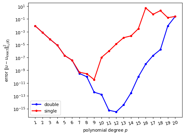
Results are shown both for single precision and double precision arithmetic. We would expect that the error decreases for higher values of $p$ since the solution can be approximated better by higher degree polynomials. Although initially this is indeed the case, it appears that the error can not be reduced below a certain value and it in fact increases for larger values of $p$. To understand this behaviour, we need to discuss how (real) numbers are represented on a computer.

Floating point numbers

A general floating point number system $\mathbb{F}$ is specified by four integer numbers:

a base $1<\beta\in\mathbb{N}$
a precision $0<p\in\mathbb{N}$
a range of exponents defined by $L,U\in\mathbb{Z}$ with $L<0\le U$

The set $\mathbb{F}$ consists of all numbers $x$ of the form

\[ x = \pm \underbrace{\left(d_0 + d_1\beta^{-1} + d_2\beta^{-2} + \dots+d_{p-1}\beta^{1-p}\right)}_{\text{mantissa}}\cdot\beta^E\qquad(25) \]

where the coefficients $d_i\in \{0,1,2,\dots,\beta-1\}$ and the exponent $E$ with $L\le E\le U$ are natural numbers. The expression in brackets is called the mantissa. Note that although $\beta,p,L,U$ as well as $E,d_i$ are integers, they represent real numbers through (25).

The floating point number system $\mathbb{F}$ is called normalised if $d_0>0$; this makes each number in $\mathbb{F}$ unique.

Example

The number $234.7$ is \[ \left(2+3\cdot 10^{-1}+4\cdot 10^{-2} +7\cdot 10^{-3}\right)\cdot 10^2 \]

in precision 4, base 10 arithmetic. It cannot be represented exactly in precision 3, base 10 arithmetic (and would have to be approximated as $\left(2+3\cdot 10^{-1}+5\cdot 10^{-2}\right)\cdot 10^2 = 235$ in this case).

The smallest positive normalised number of the from (25) is obtained by setting $d_0=1$, $d_i=0$ for $i>0$ and $E=L$. This results in $1\cdot \beta^L$ which is also is called the underflow threshold.

The largest positive normalised number in $\mathbb{F}$ is obtained by setting $d_i=\beta-1$ for $i\ge 0$ and $E=U$. This results in

\[ \begin{aligned} (\beta-1)\left(1+\beta^{-1}+\beta^{-2}+\dots+\beta^{1-p}\right)\cdot \beta^U &= (\beta-1) \beta^U \sum_{j=0}^{p-1} \beta^{-p}\\ &= (1-\beta^{-p})\beta^{U+1}, \end{aligned} \]

which is also called the overflow threshold.

Obviously, the floating point number system $\mathbb{F}$ is not closed under standard arithmetic operations: for example, $x,y\in\mathbb{F}$ does not necessarily imply that $x+y\in\mathbb{F}$. If a computation with two numbers $x,y\in\mathbb{F}$ results in a number $z\not\in\mathbb{F}$ we need to somehow represent $z$ by some nearby element $\tilde{z} := \mathcal{R}_{\mathbb{F}}(z)\in\mathbb{F}$ such that $|z-\widetilde{z}|$ is small. A common choice is to employ some sort of rounding.

IEEE 754 (Normalised) Arithmetic

The most commonly used floating point systems on modern computers are single- and double-precision, which are implemented according to the IEEE 754 standard. In both cases, $\beta=2$ and it is implicitly assumed that $d_0=1$, so this number does not have to be stored.

Single precision

np.float32: One binary digit (=bit) is used to store the sign, 8 for the exponent and 23 for the mantissa $\Rightarrow$ 32 bits (4 bytes) in total.

For single precision numbers in the IEEE 754 standard we have that

$p=24$
$L=-126$
$U=127$

which results in

Underfloat threshold = $2^{-126} \approx 10^{-38}$
Overflow threshold = $2^{128} \approx 10^{38}$

Double precision

np.float64: One binary digit is used to store the sign, 11 for the exponent and 52 for the mantissa $\Rightarrow$ 64 bits (8 bytes) in total.

For double precision numbers in the IEEE 754 standard we have that

$p=53$
$L=-1022$
$U=1023$

which results in

Underfloat threshold = $2^{-1022} \approx 10^{-308}$
Overflow threshold = $2^{1024} \approx 10^{308}$

Representation of special values

Since $d_0=1$ it appears that we can not store the number zero. To represent this number and some other special cases, several dedicated bit patterns are reserved:

The number zero is stored as s000 0000 0000 0000 0000 0000 0000 0000 where $s$ is the sign bit. Note that there is both $+0$ ($s=1$) and $-0$ ($s=0$).
NaN (“not a number”) is stored as s111 1111 1xxx xxxx xxxx xxxx xxxx xxxx where the sequence denoted with $x$ stands for any non-zero number and the sign $s$ is usually ignored. The result of mathematically invalid operations (such as taking the square root of a negative number) is stored as a NaN
Infinity ($\pm\infty$) is stored as s111 1111 1000 0000 0000 0000 0000 0000 where again $s$ denotes the sign. This result can arise from division by zero.

Machine epsilon

From (25) it can be seen that gaps between numbers in $\mathbb{F}$ increase for larger numbers. For each exponent $E$ the interval $[2^E,2^{E+1}]$ is discretised into $2^{p-1}$ equal pieces of size $2^{1-p}\cdot 2^E$, as shown in the following figure:

Figure 10: floating point number spacing

Setting $E=0$, we see that the size of gap of numbers in $\mathbb{F}$ around $1$ is

\[ 2^{1-p} = \begin{cases} 2^{-23} \approx 10^{-7} & \text{in single precision}\\ 2^{-52} \approx 2\cdot 10^{-16} & \text{in double precision} \end{cases} \]

This quantity is also known as the machine epsilon $\varepsilon_{\text{mach}}$. It is the smallest positive number $x\in \mathbb{F}$ that can be added to $1$ such that (after rounding to $\mathbb{F}$) the result is different from $1$:

\[ \varepsilon_{\text{mach}} := \min_{x\in\mathbb{F},x>0}\{x: \mathcal{R}_{\mathbb{F}}(1+x)\neq 1\} \qquad(26) \]

Put differently, the machine epsilon is the relative size of rounding errors or the relative accuracy of floating point operations. If $z$ is the result of some arithmetic operation involving numbers from $\mathbb{F}$ then

\[ \frac{|\mathcal{R}_{\mathbb{F}}(z)-z|}{|z|} \sim \varepsilon_{\text{mach}}. \]

Rounding errors

As the following examples show, rounding errors can have serious consequences

Example 1 (harmless)

Consider the two numbers $x=4.7\cdot 10^{-16}$ and $y=2.9\cdot 10^{-16}$. Both can be represented exactly as floating point numbers. The same is true for their difference $z=x-y=1.8\cdot 10^{-16}$, i.e. $\widetilde{z}=\mathcal{R}_{\mathbb{F}}(z)=z$ and as a consequence the rounding error of this operation is zero:

\[ \frac{\mathcal{R}_{\mathbb{F}}(z)-z}{z} = \frac{\mathcal{R}_{\mathbb{F}}(x)-\mathcal{R}_{\mathbb{F}}(y)-z}{z} = \frac{(4.7 -2.9 - 1.8)\cdot10^{-16}}{1.8\cdot 10^{-16}} = 0. \] In general, adding or subtracting numbers leads to small relative errors provided both the numbers and the result of the computation are of comparable size. As the following example shows, the final point is crucial.

Example 2 (subtracting two numbers that are very close)

Now assume that we compute the difference of the two numbers $x=4.7\cdot 10^{-16}$, $x=2.9\cdot 10^{-16}$ by first adding $x$ and $y$ to one and then subtract the resulting numbers: $x'=1+x$, $y'=1+y$, $z'=x'-y'$. Although in exact arithmetic $z'$ will be identical to $x-y$, this is not true in floating point arithmetic. First observe that in double precision arithmetic $x'$ will be rounded to $\mathcal{R}_{\mathbb{F}}(x')=1.00000000000000044$ and $y'$ will be rounded to $\mathcal{R}_{\mathbb{F}}(y')=1.00000000000000022$. The relative error of $z'$ is:

\[ \frac{\mathcal{R}_{\mathbb{F}}(z')-z}{z} = \frac{\mathcal{R}_{\mathbb{F}}(x')-\mathcal{R}_{\mathbb{F}}(y')-z}{z} = \frac{(4.4 - 2.2 - 1.8)\cdot10^{-16}}{1.8\cdot 10^{-16}} = \frac{0.4}{1.8} \approx 23\% \]

Example 3 (adding two numbers of very different size)

Consider the linear system \[ \begin{pmatrix} 0 & 1 \\ 1 & 1 \end{pmatrix} \begin{pmatrix} x_0 \\ x_1 \end{pmatrix} = \begin{pmatrix} 1 \\ 0 \end{pmatrix}. \] The solution is $x_0=-1$, $x_1=+1$. Now consider a small perturbation of this problem, namely \[ \begin{pmatrix} -10^{-20} & 1 \\ 1 & 1 \end{pmatrix} \begin{pmatrix} x_0 \\ x_1 \end{pmatrix} = \begin{pmatrix} 1 \\ 0 \end{pmatrix}\qquad(27) \] It is easy to see that the solution of the perturbed problem is $x_0=-\frac{1}{1+10^{-20}}$, $x_1=+\frac{1}{1+10^{-20}}$, which is very close to the solution of the unperturbed system.

Let us solve the perturbed system in (27) numerically. For this, we write it as

\[ \begin{aligned} -10^{-20} x_0 + x_1 &= 1\\ x_0 + x_1 &= 0 \end{aligned} \] To eliminate $x_0$ from the second equation, we multiply the first equation with $10^{20}$ and add it to the second equation to obtain \[ \begin{aligned} -10^{-20} x_0 + x_1 &= 1\\ (1+10^{20}) x_1 &= 10^{20} \end{aligned} \] Now, since $10^{20}\gg 1$, we can replace $1+10^{20}$ by $10^{20}$ (and this is what will happen in double precision arithmetic) to obtain \[ \begin{aligned} -10^{-20} x_0 + x_1 &= 1\\ 10^{20} x_1 &= 10^{20}, \end{aligned} \] which immediately implies $x_1 = 1$. Inserting this into the first equation gives \[ \begin{aligned} -10^{-20} x_0 + 1 &= 1 \end{aligned} \] and therefore $x_0=0$. Altogether we find $x_0=0$, $x_1=1$. This is very different from the exact solution $x_0=-\frac{1}{1+10^{-20}}$, $x_1=+\frac{1}{1+10^{-20}}$! Hence, although the rounding we performed in the numerical solution procedure appears to be innocent, we get a completely wrong solution. In this case, this problem can be fixed by using a slightly different solution procedure: subtract the first equation from the second equation to obtain $(1+10^{-20}) x_0 = -1$, which can be safely approximated by $x_0=-1$. Then use this in the second equation $x_0+x_1=0$ to conclude $x_1=+1$. Now this is very close to the exact solution of the perturbed system. It turns out that solving the perturbed linear system with np.linalg.solve() will also give a good approximation. Unfortunately, this is not always the case, as the following example demonstrates.

Example 4 (ill-conditioned matrix)

For a given positive $\epsilon>0$ consider the following $2\times 2$ symmetric matrix

\[ \begin{aligned} A &= \begin{pmatrix} 1+\frac{1}{\sqrt{2}} + \frac{2+\sqrt{2}}{4}\epsilon & \frac{1}{\sqrt{2}}-\frac{\sqrt{2}}{4}\epsilon\\[1ex] \frac{1}{\sqrt{2}}-\frac{\sqrt{2}}{4}\epsilon & 1-\frac{1}{\sqrt{2}}+\frac{2-\sqrt{2}}{4}\epsilon \end{pmatrix} \\ &\approx \begin{pmatrix} 1.7071067811865475 + 0.8535533905932737 \cdot\epsilon & 0.7071067811865475 - 0.3535533905932738 \cdot\epsilon \\ 0.7071067811865475 - 0.3535533905932738 \cdot\epsilon & 0.2928932188134525 + 0.1464466094067262\cdot\epsilon \end{pmatrix} \end{aligned}\qquad(28) \]

and vector

\[ \boldsymbol{b} = \begin{pmatrix} \frac{\sqrt{2+\sqrt{2}}+\sqrt{2-\sqrt{2}}}{2}\\[1ex] \frac{\sqrt{2+\sqrt{2}}-\sqrt{2-\sqrt{2}}}{2} \end{pmatrix} \approx \begin{pmatrix} 1.3065629648763766\\0.5411961001461970 \end{pmatrix}\qquad(29) \]

It can be shown that independent of $\epsilon$ the exact solution of the linear system $A\boldsymbol{u}=\boldsymbol{b}$ with $A$ in @eqn:constructed_A and $\boldsymbol{b}$ in (29) is given by

\[ \boldsymbol{u}_{\text{exact}} = \begin{pmatrix} \frac{\sqrt{2 - \sqrt{2}}}{2}\\[1ex] \frac{\sqrt{2 + \sqrt{2}}}{2} \end{pmatrix} \approx \begin{pmatrix} 0.3826834323650897\\0.9238795325112867 \end{pmatrix} \]

Hence, we would expect that if we solve the linear system with a numerical method, we would get a solution that is at least close to the exact solution. The following table shows the solution $\boldsymbol{u}$ of $A\boldsymbol{u}=\boldsymbol{b}$ that is obtained with

u = np.linalg.solve(A,b)

for different values of $\epsilon$. The pen-ultimate column shows the relative error $\|\boldsymbol{u}-\boldsymbol{u}_{\text{exact}}\|_2|/\|\boldsymbol{u}_{\text{exact}}\|_2$ and the final column shows the condition number $\kappa = \text{cond}(A) = \lambda_+/\lambda_-$, which is the ratio of the largest and smallest eigenvalue of $A$.

$\epsilon$	solution $\boldsymbol{u}$	relative error $\\|\\|\boldsymbol{u}-\boldsymbol{u}_{\text{exact}}\\|\\|_2/\\|\\|\boldsymbol{u}_{\text{exact}}\\|\\|_2$	condition number $\kappa$
$10^{-3}$	$\begin{pmatrix}0.3826834323650560 \\ 0.9238795325113685\end{pmatrix}$	$8.8408\cdot 10^{-14}$	$4\cdot 10^3$
$10^{-6}$	$\begin{pmatrix}0.3826834323171860 \\0.9238795326269368\end{pmatrix}$	$1.2518\cdot 10^{-10}$	$4\cdot 10^6$
$10^{-9}$	$\begin{pmatrix}0.3826834290672392 \\0.9238795404730024\end{pmatrix}$	$8.6177\cdot 10^{-9}$	$4\cdot 10^9$
$10^{-12}$	$\begin{pmatrix}0.3826776593455781 \\ 0.9238934698132879\end{pmatrix}$	$1.5086\cdot10^{-5}$	$4\cdot 10^{12}$
$10^{-15}$	$\begin{pmatrix}0.3888090807546386 \\0.9090909090909092\end{pmatrix}$	$1.6007\cdot10^{-2}$	$4\cdot 10^{15}$
$8\cdot 10^{-16}$	$\begin{pmatrix} 0.2919799363037854 \\1.1428571428571428\end{pmatrix}$	$2.3702\cdot 10^{-1}$	$5\cdot 10^{15}$
$4\cdot 10^{-16}$	$\begin{pmatrix} -0.0630602600160104 \\ 2.0000000000000000\end{pmatrix}$	$1.1648$	$10^{16}$

Clearly, the errors increase for smaller values of $\epsilon$. This is related to the growth of condition number of the matrix. The two eigenvalues of $A$ are

\[ \lambda_{\pm} = 1+\frac{\epsilon}{2}\pm\sqrt{1-\frac{\epsilon^2}{4}} \approx \{2,\frac{\epsilon}{2}\} \qquad\text{for $\epsilon\ll 1$} \]

and hence the condition number is

\[ \kappa = \frac{\lambda_+}{\lambda_-} = \frac{1+\frac{\epsilon}{2}+\sqrt{1-\frac{\epsilon^2}{4}}}{1+\frac{\epsilon}{2}-\sqrt{1-\frac{\epsilon^2}{4}}} \approx \frac{4}{\epsilon} \]

It appears that matrices with large condition numbers cause problems.

Backward error analysis

In general, when solving linear systems with $n$ equations we are interested in quantifying the error on the solution.

In exact arithmetic the solution $\boldsymbol{u}\in\mathbb{R}^n$ satisfies

\[ A\boldsymbol{u} = \boldsymbol{b} \]

where $A$ is a $n\times n$ matrix. However, due to rounding errors, the solution $\boldsymbol{u}'=\boldsymbol{u}+\delta\boldsymbol{u}$ that we actually compute corresponds to the solution of the perturbed system

\[ (A+\delta A)(\boldsymbol{u}+\delta\boldsymbol{u}) = \boldsymbol{b} + \delta\boldsymbol{b} \]

If we set $\delta\boldsymbol{b}=0$ for the moment, we can derive a bound on $\delta\boldsymbol{u}$ for the case where Gaussian elimination is used to solve the linear system. For this we use the following norm on vectors and matrices:

\[ \begin{aligned} \|\boldsymbol{w}\|_\infty &:= \max_{i=0,\dots,n-1} |w_i|,\\ \|A\|_\infty &:= \max_{\boldsymbol{w}\in\mathbb{R}^n,\boldsymbol{w}\neq \boldsymbol{0}} \frac{\|A\boldsymbol{w}\|_\infty}{\|\boldsymbol{w}\|_\infty} = \max_{0\le i < n} \sum_{j=0}^{n-1} |A_{ij}| \end{aligned} \]

Using the definition, it is easy to see that $\|A\boldsymbol{w}\|_\infty\le \|A\|_\infty\|\boldsymbol{w}\|_\infty$ and $\|AB\|_\infty\le\|A\|_\infty\|B\|_\infty$.

The condition number of a matrix $A$ is given by

\[ \text{cond}(A) := \|A^{-1}\|_\infty\|A\|_\infty. \]

(For a real-valued symmetric positive matrix this is identical to the ratio of the largest and smallest eigenvalue).

We now have the following

Theorem 1

If the $n\times n$ matrix $A$ is non-singular and $\delta A$ is sufficiently small, namely

\[ \|\delta A\|_{\infty} \|A^{-1}\|_\infty \le \frac{1}{2} \]

then $A+\delta A$ is non-singular and

\[ \frac{\|\delta\boldsymbol{u}\|_\infty}{\|\boldsymbol{u}\|_\infty} \le 2\text{cond}(A) \frac{\|\delta A\|_\infty}{\|A\|_\infty}. \qquad(30) \]

The bound in (30) is derived below. Furthermore, it can be shown that if Gaussian elimination is used to solve the linear system (and this is the method used by numpy.linalg.solve), then the effect of roundoff errors is

\[ \frac{\|\delta A\|_\infty}{\|A\|_\infty} \le n \varepsilon_{\text{mach}} G(A), \]

where $G(A)$ is a “well-behaved” number that depends on the matrix $A$ and $\varepsilon_{\text{mach}}$ is the machine epsilon defined in (26). Although it is possible to construct pathological examples for which $G(A)$ is large, it is reasonable to assume that for the matrices that we consider here $G(A)$ is small and only depends weakly on $A$. Putting everything together, we find that

Theorem 2

Under the conditions of Theorem 1 and if Gaussian elimination is used to solve the linear system, the error $\delta \boldsymbol{u}$ can be bounded

\[ \frac{\|\delta\boldsymbol{u}\|_\infty}{\|\boldsymbol{u}\|_\infty} \le 2G(A)\cdot n\cdot \text{cond}(A)\cdot \varepsilon_{\text{mach}}. \]

Summary

Although this is only an upper bound which does not necessarily have to be tight, this result implies that the (relative) error $\|\delta\boldsymbol{u}\|_\infty/\|\boldsymbol{u}\|_\infty$

is proportional to the machine epsilon $\varepsilon_{\text{mach}}$ defined in (26),
increases with problem size $n$,
and grows with the condition number $\text{cond}(A)$ of the matrix.

These observations explain the behaviour seen in Figure 7: the size of the matrix and its condition number increase for higher polynomial degrees, as shown in Figure 11. The error can be reduced by using double precision ($\varepsilon_{\text{mach}}\sim 10^{-16}$) instead of single precision ($\varepsilon_{\text{mach}}\sim 10^{-7}$). It is also possible to reduce the condition number by using a better placement of the points $\xi^{(\ell)}$ which define the basis functions, but we will not pursue this here since we are typically only interested in relatively low polynomial degrees $p$ where this is not an issue.

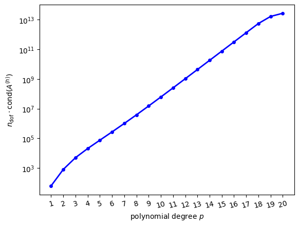
Figure 11: Product of problem size n_{\text{dof}} and condition number \text{cond}(A^{(h)}) — Figure 11: Product of problem size $n_{\text{dof}}$ and condition number $\text{cond}(A^{(h)})$

Unfortunately, the problems that are generally encountered in Scientific Computing are usually large ($n\gg 1$) and characterised by ill-conditioned matrices. Observe further that while in the examples above we were able to quantify the error by comparing the numerical solution to the exact solution, this is usually not possible: in most cases we do not even know how large the error is!

Estimating the error

In general it is not possible to compute the error $\delta\boldsymbol{u}$. However, since $\boldsymbol{b}-A\boldsymbol{u}=0$, it is natural to consider the residual $\boldsymbol{r}:=\boldsymbol{b}-A\boldsymbol{u}'$ which measures to which degree the numerical solution $\boldsymbol{u}'=\boldsymbol{u}+\delta\boldsymbol{u}$ fails to satisfy the linear system. Unfortunately, if $\|\boldsymbol{r}\|_\infty$ is small this does not necessarily imply the smallness of the error $\|\delta\boldsymbol{u}\|_\infty$. To see this, first observe that $\boldsymbol{r}=A\delta\boldsymbol{u}$. Then note that since $\|\boldsymbol{b}\|_\infty \le \|A\|_\infty \|\boldsymbol{u}\|_\infty$ and $\|\delta\boldsymbol{u}\|_\infty \le \|A^{-1}\|_\infty \|\boldsymbol{r}\|_\infty$

\[ \frac{\|\delta \boldsymbol{u}\|_\infty}{\|\boldsymbol{u}\|_\infty} \le \|A^{-1}\|_\infty\| \boldsymbol{r}\|_\infty \frac{\|A\|_\infty}{\|\boldsymbol{b}\|_\infty}\\ = \text{cond}(A)\frac{\|\boldsymbol{r}\|_\infty}{\|\boldsymbol{b}\|_\infty} \]

Hence, the smallness of $\|\boldsymbol{r}\|_\infty/\|\boldsymbol{b}\|_\infty$ only implies the smallness of the relative error $\|\delta \boldsymbol{u}\|_\infty/\|\boldsymbol{u}\|_\infty$ if the condition number of $A$ is small. Nevertheless, in the absence of any other information on the error, the residual $\|\boldsymbol{r}\|_\infty$ is a very useful quantity to measure.

Proof of Theorem 1 (not examinable)

Observe first that if $X$ is any $n\times n$ real-valued matrix with $\|X\|_\infty<1$ then $\|X^n\|_\infty\le \|X\|_\infty^n\rightarrow 0$ as $n\rightarrow\infty$. Thus

\[ (I-X)(1+X+X^2+\dots+X^n) = 1-X^{n+1} \rightarrow I\quad\text{as $n\rightarrow\infty$}. \]

This implies that

\[ (I-X)^{-1}=\sum_{j=0}^{\infty} X^j \]

and

\[ \|(I-X)^{-1}\|_\infty \le \sum_{j=0}^{\infty} \|X^j\|_\infty \le \sum_{j=0}^{\infty} \|X\|_\infty^j = (1-\|X\|_\infty)^{-1} \qquad(31) \]

Now write

\[ A + \delta A = (I+\delta A\;A^{-1})A \]

and set $X=-\delta A\;A$. By the assumption $\|X\|_\infty\le \frac{1}{2}<1$ and we can apply (31) to show that $I+\delta A\;A^{-1}$ is non-singular and that

\[ \|(I+\delta A\;A)^{-1}\|_\infty\le (1-\|\delta A\;A^{-1}\|_\infty)^{-1} \le 2. \]

As a consequence, $A+\delta A$ is non-singular and

\[ \|(A+\delta A)^{-1}\|_\infty = \|A^{-1}(I+\delta A\;A^{-1})^{-1}\|_\infty \le 2\|A^{-1}\|_\infty \]

Finally, subtract the two equations $(A+\delta A)(\boldsymbol{u}+\delta\boldsymbol{u})=\boldsymbol{b}$ and $A\boldsymbol{u}=\boldsymbol{b}$ to obtain $(A+\delta A)\delta\boldsymbol{u} = -\delta A \boldsymbol{u}$. After multiplication by the inverse of $A+\delta A$ this becomes

\[ \delta\boldsymbol{u} = (A+\delta A)^{-1}\delta A\boldsymbol{u}. \]

Taking the norm leads to

\[ \begin{aligned} \|\delta \boldsymbol{u}\|_\infty &\le \|(A+\delta A)^{-1}\|_\infty \|\delta A\|_\infty \|\boldsymbol{u}\|_\infty\\ &\le 2 \underbrace{\|A^{-1}\|_\infty\|A\|_\infty}_{=\text{cond}(A)} \frac{\|\delta A\|_\infty}{\|A\|_\infty}\|\boldsymbol{u}\|_\infty \end{aligned} \]

To finish the proof, divide both sides of this inequality by $\|\boldsymbol{u}\|_\infty$ to obtain (30).

Unstructured meshes

So far, we have only solved our model PDE on a very simple domain, consisting of a single reference triangle. We now discuss how to extend the finite element approach to more general domains, using the concepts introduced in [CH24]. Assume that we want to solve the PDE on a $d$-dimensional manifold $\Omega\subset \mathbb{R}^D$ that is embedded in $D$ dimensional space. For example, we might want to solve it in a rectangular domain or on the surface of a sphere. The manifold is then approximated by a mesh, which can be described as a collection of topological entities. For example, if $d=2$, the mesh will consist of zero-dimensional vertices, one-dimensional edges and two-dimensional triangular cells (although it is also possible to use more general polygonal cells we do not consider this here). In general, the co-dimension $c$ of a $d'$-dimensional mesh entity is given by $c=d-d'$. In the following we will only consider the case $d=D=2$, but the central ideas that are developed in the following also apply to more complicated setups. For $d=D=2$ we have:

topological entity	dimension $d'$	co-dimension $c$
cell (triangle) $K$	$2$	$0$
facet (edge) $F$	$1$	$1$
vertex (point) $v$	$0$	$2$

Figure 12 shows a two-dimensional mesh with $n_{\text{vertex}}=6$ vertices, $n_{\text{facet}}=10$ facets and $n_{\text{cell}}=5$ cells in which all topological entities are labelled by their co-dimension and a unique number that can later be used to identify the entity.

Topology

The mesh topology describes which entities are connected to which other entities. For example, each cell has exactly three facets and each facet is defined by exactly two vertices, and the topology tells us which specific facets/vertices these are: in the example above, cell $(0,1)$ has the facets $(1,3), (1,2), (1,5)$ and facet $(1,2)$ has the endpoints $(2,1), (2,2)$.

More generally, this information can be encoded in two matrices: An $n_{\text{cell}}\times 3$ matrix $I^{K\rightarrow F}$ which describes which facets bound each cell

\[ I^{K\rightarrow F}_{\alpha\beta} = \text{index of $\beta$-th facet of cell $\alpha$} \]

and an $n_{\text{facet}}\times 2$ matrix $I^{F\rightarrow v}$ which describes what the endpoints of each facet are

\[ I^{F\rightarrow v}_{\beta\gamma} = \text{index of $\gamma$-th vertex of facet $\beta$}. \]

Note that there is some freedom as to how we number the facets associated each cell; the numbering we adopt here is one in which for each cell $\alpha$ the facets with indices $I^{K\rightarrow F}_{\alpha0}$, $I^{K\rightarrow F}_{\alpha1}$ and $I^{K\rightarrow F}_{\alpha2}$ are arranged in a counter-clockwise fashion (note that there are three possible orderings that satisfy this condition, so we have to pick one). Similarly, we adapt an ordering of the vertices associated with each facet such that for each facet $\beta$ we have that $I^{F\rightarrow v}_{\beta0} < I^{F\rightarrow v}_{\beta1}$; in Figure 12 this is indicated by the arrows on the edges.

For convenience, we can also use $I^{K\rightarrow F}$ and $I^{F\rightarrow v}$ to construct the $n_{\text{cell}}\times 3$ matrix $I^{K\rightarrow v}$ which describes the vertices of a given cell

\[ I^{K\rightarrow v}_{\alpha\gamma} = \text{index of $\gamma$-th vertex of cell $\alpha$}. \]

In each cell $\alpha$, we number the vertices in a counter-clockwise fashion such that the $\gamma$-th vertex lies opposite the $\gamma$-the facet of the cell. Mathematically, this can be expressed as

\[ \begin{aligned} I^{K\rightarrow v}_{\alpha\gamma} \not\in \{I^{F\rightarrow v}_{\beta0},I^{F\rightarrow v}_{\beta1}\}\quad\text{for $\beta =I^{K\rightarrow F}_{\alpha\gamma}$} \end{aligned}. \]

Note that the counter-clockwise numbering of the facets and vertices in each cell is consistent with the numbering of unknowns on the reference triangle in Figure 3.

For example, the matrices $I^{K\rightarrow F}$, $I^{F\rightarrow v}$ and $I^{K\rightarrow v}$ for the simple mesh shown above are given by

\[ \begin{aligned} I^{K\rightarrow F} &= \begin{pmatrix} 0 & 3 & 1 & 0 & 3 \\ 1 & 2 & 2 & 9 & 6 \\ 8 & 5 & 7 & 5 & 4 \end{pmatrix}^{\top}\\ I^{F\rightarrow v} &= \begin{pmatrix} 0 & 1 & 1 & 2 & 2 & 1 & 3 & 2 & 0 & 0 \\ 1 & 4 & 2 & 5 & 3 & 5 & 5 & 4 & 4 & 5 \end{pmatrix}^{\top}\\ I^{K\rightarrow v} &= \begin{pmatrix} 4 & 1 & 2 & 5 & 3 \\ 0 & 5 & 4 & 1 & 2 \\ 1 & 2 & 1 & 0 & 5 \end{pmatrix}^{\top} \end{aligned} \]

You should convince yourself that these matrices satisfy the conditions outlined above.

Figure 13 shows another example (created with rectangle_mesh(Lx=1.0, Ly=1.0, nref=1), see below). The global indices of vertices, facets and cells are plotted separatedly. The figure in the lower right corner illustrates how the global indices are related to the local indices of the reference cell.

Figure 13: Numbering of topological entities on a rectangle mesh

Referring to the local numbering of facets and vertices in the lower right plot we read off:

\[ \begin{aligned} I^{K\rightarrow F} &= \begin{pmatrix} 5 & 1 & 2 & 10 & 8 & 0 & 7 & 13\\ 0 & 3 & 4 & 11 & 1 & 6 & 9 & 14\\ 11 & 12 & 10 & 12 & 14 & 15 & 13 & 15 \end{pmatrix}^{\top} \\ I^{F\rightarrow v} &= \begin{pmatrix} 1 & 2 & 0 & 2 & 0 & 1 & 1 & 3 & 2 & 3 & 5 & 4 & 4 & 7 & 4 & 4\\ 4 & 4 & 5 & 5 & 6 & 6 & 7 & 7 & 8 & 8 & 6 & 6 & 5 & 8 & 8 & 7 \end{pmatrix}^{\top} \\ I^{K\rightarrow v} &= \begin{pmatrix} 4 & 5 & 6 & 4 & 4 & 7 & 8 & 4\\ 6 & 4 & 5 & 5 & 8 & 4 & 7 & 7\\ 1 & 2 & 0 & 6 & 2 & 1 & 3 & 8 \end{pmatrix}^{\top} \end{aligned} \]

Again, convince yourself that these matrices are consistent with the conditions we imposed on the numbering.

Implementation

The class Mesh in fem/mesh.py encodes the mesh topology. It has the following members:

properties ncells, nfacets and nvertices which give the total number of cells ($=n_{\text{cell}}$), facets ($=n_{\text{facet}}$) and vertices ($=n_{\text{vertex}}$) respectively
cell2facet: a nested list such that cell2facet[alpha][beta] $= I^{K\rightarrow F}_{\alpha\beta}$
facet2vertex: a nested list such that facet2vertex[beta][gamma] $= I^{F\rightarrow v}_{\beta\gamma}$
cell2vertex: a nested list such that cell2vertex[alpha][gamma] $= I^{K\rightarrow v}_{\alpha\gamma}$. Since $I^{K\rightarrow v}_{ik}$ can be derived from $I^{K\rightarrow F}_{\alpha\beta}$ and $I^{F\rightarrow v}_{\beta\gamma}$, cell2vertex is implemented as a @functools.cached_property.
an array coordinates of shape $(n_{\text{vertex}},2)$ whose columns contain the two-dimensional coordinates of the mesh vertices

The class also contains a method refine(nref) which can be used to construct a refined mesh from a given mesh by sub-dividing each triangle into four smaller triangles.

In fem/utilitymeshes.py two factory classes are defined which returns specific meshes:

rectangle_mesh(Lx=1.0, Ly=1.0, nref=0) is a triangulation of the domain $[0,L_x]\times[0,L_y]$ with a given number of refinements $n_{\text{ref}}$. The number of cells is $n_{\text{cells}} = 2^{n_{\text{ref}}+1}$
triangle_mesh(corners=None, nref=0) is a triangulation of the domain triangle defined by the array corners (if this is None, the reference triangle us used) with a given number of refinements $n_{\text{ref}}$. The number of cells is $n_{\text{cells}} = 2^{n_{\text{ref}}}$

Geometry

Observe that so far we have only discussed the topology of the mesh and we have not said anything about its geometry, i.e. where exactly the topological entities are located in space. To do this, we first discuss how we can associate data with the mesh and then use this to encode its geometry.

Function spaces

Grid cells and reference elements

We now construct a function space $\mathcal{V}_h\subset H^1(\Omega_h)$ on the domain $\Omega_h$ defined by the mesh as follows. First, we assume that each cell $K$ of the mesh is the image of the reference cell $\widehat{K}$ under a bijective map $X_K:\widehat{K}\rightarrow K\subset \Omega\subset \mathbb{R}^2$: for each $\widehat{x}\in\widehat{K}$ there is exactly one point $x=X_K(\widehat{x})\in K$ and vice versa. For an arbitrary real-valued function $f:K\rightarrow \mathbb{R}$ we define the pullback $\widehat{f}:\widehat{K}\rightarrow \mathbb{R}$ under $X_K$ as

\[ \widehat{f} = f\circ X_K \]

i.e.

\[ \widehat{f}(\widehat{x}) = f(X_K(\widehat{x}))\qquad\text{for all $\widehat{x}\in\widehat{K}$}. \]

Next, assume that in each grid cell $K$ the pullback of the function $u|_K$ under the map $X_K$ is a polynomial. More specifically we define \[ \mathcal{V}_h := \{u\in H^1(\Omega_h): u|_K(x) = \widehat{u}_K(\widehat{x})\quad \text{for some $\widehat{u}_K\in\mathcal{P}_p(\widehat{K})$ with $x=X_K(\widehat{x})$ for all cells $K\in\Omega_h$}\}. \]

Figure 14: pullback to reference element

We can now use the basis of $\mathcal{P}_p(\widehat{K})$ that we constructed in one of the previous lectures to represent the functions $\widehat{u}_K$. However, care has to be taken to ensure that the function $u\in\mathcal{V}_h$ defined on the entire domain is continuous across facets and at the vertices. To guarantee this, we need to think carefully about the arrangement of unknowns on the mesh.

For this, recall that any function $u_h$ in the function space $\mathcal{V}_h$ can be written as

\[ u_h(x) = \sum_{\ell_{\text{global}}=0}^{n-1} u^{(h)}_{\ell_{\text{global}}} \Phi^{(h)}_{\ell_{\text{global}}}(x) \]

where the $\Phi^{(h)}_{\ell_{\text{global}}}$ are the global basis functions and $u^{(h)}_{\ell_{\text{global}}}$ are entries of the global dof-vector $\boldsymbol{u}^{(h)}$. To ensure continuity of $u_h$ we need to associate the indices $\ell_{\text{global}}$ with the correct mesh entities.

Arrangement of unknowns

Assume that we have a finite element with $\nu_{\text{vertex}}$ unknowns per vertex, $\nu_{\text{facet}}$ unknowns per facet and $\nu_{\text{interior}}$ unknowns per cell. Let $N_{\text{vertex}} = n_{\text{vertex}}\cdot \nu_{\text{vertex}}$, $N_{\text{facet}} = n_{\text{facet}}\cdot \nu_{\text{facet}}$ and $N_{\text{interior}} = n_{\text{cell}}\cdot \nu_{\text{interior}}$ be the total number of unknowns associated with vertices, facets and cell interiors respectively.

We number the unknowns by using the first $N_{\text{vertex}}$ indices for unknowns associated with vertices, the next $N_{\text{facet}}$ indices for unknowns associated with facets and the remaining $N_{\text{interior}}$ indices for unknowns associated with cell interiors. More specifically:

unknowns with indices $\ell_{\text{global}}\in\{\gamma\cdot \nu_{\text{vertex}},\dots,(\gamma+1)\cdot \nu_{\text{vertex}}-1\}$ are associated with the $\gamma$-th vertex
unknowns with indices $\ell_{\text{global}}\in\{N_{\text{vertex}}+\beta\cdot \nu_{\text{facet}},\dots,N_{\text{vertex}}+(\beta+1)\cdot \nu_{\text{facet}}-1\}$ are associated with the $\beta$-th facet
unknowns with indices $\ell_{\text{global}}\in\{N_{\text{vertex}}+N_{\text{facet}}+\alpha\cdot \nu_{\text{interior}},\dots,N_{\text{vertex}}+N_{\text{facet}}+(\alpha+1)\cdot \nu_{\text{interior}}-1\}$ are associated with the $\alpha$-th cell

The facet-unknowns are ordered along the orientation of each edge.

Figure 15 shows an example for the $p=3$ Lagrange element. For this mesh there are $N_{\text{vertex}}=6$ unknowns associated with the vertices, $N_{\text{facet}}=10\cdot 2=20$ unknowns associated with the facets and $N_{\text{interior}} = 5$ unknowns associated with the cell interiors.

Figure 15: simple triangular mesh with unknowns

Local-to-global map

When we introduced the concept of a finite element, we only considered local basis functions $\phi_\ell$. Since the functions in $\mathcal{V}_h$ are continuous, the global basis functions $\Phi^{(h)}_{\ell_{\text{global}}}$ are a combination of local basis functions: for example, global functions associated with a vertex are a combination of local basis functions on the cells that touch this vertex. Hence, in general the dof-index $\ell_{\text{global}}$ is related to several pairs $(\alpha,\ell)$ of cell indices $\alpha$ and local dof-indices $\ell$.

Conversely, on each cell with index $\alpha$ we need to map the $\ell$-th local dof-index to the global dof-index $\ell_{\text{global}}$. Note that this map is surjective but not injective since the unknowns associated with the facets and vertices are shared.

The map $(\alpha,\ell) \mapsto \ell_{\text{global}}$ is realised in two steps:

For the given $\ell$, we first work out the entity-type $E$ (cell, facet or vertex) it is associated with, as well as the index $\rho$ of this entity on the reference triangle and the index $j$ of the dof on that reference entity. Recall that for the finite element we have the dof-map $\mu_{\text{dof}}$ that $\ell = \mu_{\text{dof}}(E,\rho,j)$, so we can obtain $E$, $\rho$ and $j$ from the inverse of this map, which is implemented as the inverse_dofmap() method in the FiniteElement base class in fem/finiteelement.py.
Next, we map the tuple $(E,\rho,j)$ to the global dof index $\ell_{\text{global}}$ taking into account the arrangement of unknowns described above:
1. If $E=\text{vertex}$: $\ell_{\text{global}} = \gamma\cdot \nu_{\text{vertex}}+j$ where $\gamma=I^{K\rightarrow v}_{\alpha\rho}$ is the global index of the vertex with local index $\rho$.
2. If $E=\text{facet}$: $\ell_{\text{global}} = N_{\text{vertex}}+\beta\cdot \nu_{\text{facet}}+\widetilde{j}$ where $\beta=I^{K\rightarrow F}_{\alpha\rho}$ is the global index of the facet with local index $\rho$. Note that the orientation of the facet does not necessarily match the orientation on the reference element $\widehat{K}$. To take this into account, set $\widetilde{j}=j$ if the orientations agree and set $\widetilde{j} = \nu_{\text{facet}}-1-j$ otherwise.
3. If $E=\text{cell}$: $\ell_{\text{global}} = N_{\text{vertex}}+N_{\text{facet}}+\alpha\cdot \nu_{\text{interior}}+j$ ($\rho$ is ignored in this case)

Implementation in Python

Function spaces

The necessary functionality is implemented in the FunctionSpace class in fem/functionspace.py. The initialiser is passed a mesh and a finiteelement and the class provides the following functionality:

The property ndof contains the total number of unknowns in the function space
The method local2global(self, alpha, ell) implements the map $(\alpha,\ell)\mapsto\ell_{\text{global}}$ described above. If the parameter ell is a single integer index in the range $0,1,\dots,\nu-1$, the method returns a single number $\ell_{\text{global}}$. If ell is an iterable (such as a list [0,3,4] or range(1,6,2)) the global index will be computed for each local index and the method returns a list.

Functions

To store functions in a given function space, the class Function in fem/function.py is provided. This initialiser of this class gets passed a FunctionSpace object, which it stores together with a numpy array function.data that contains the vector $\boldsymbol{u}^{(h)}$. This information then allows the reconstruction of the function $u_h \in \mathcal{V}_h$ given by

\[ u_h(x) = \sum_{\ell_{\text{global}}=0}^{N-1} u^{(h)}_{\ell_{\text{global}}} \Phi^{(h)}_{\ell_{\text{global}}}(x) \]

To store co-functions such as $b(\cdot)\in\mathcal{V}_h^*$ with (for example)

\[ b(v) = \int_\Omega v(x) f(x)\;dx \]

a CoFunction class is provided in the same file. This class is also constructed by passing it a FunctionSpace object, but now the cofunction.data array contains the vector $\boldsymbol{b}^{(h)}$ whose elements are given by

\[ b^{(h)}_{\ell_{\text{global}}} = b\left(\Phi^{(h)}_{\ell_{\text{global}}}\right). \]

Encoding geometry information

The geometry of the mesh is encoded in the functions $X_K$ which describe the mapping from the reference element $\widehat{K}$ to a particular cell $K$. We can combine the $X_K$ in each cell into a global function $X$ which is defined on the entire mesh. The crucial observation is now that each component of $X_K$ can be represented by a function in a finite element space $\mathcal{W}_h$ which is defined in the same way as $\mathcal{V}_h$ (but possibly with a different polynomial degree). Hence, we can define a coordinate function

\[ X \in \mathcal{W}_h^{\times} = \mathcal{W}_h \times \mathcal{W}_h \] which encodes the mesh geometry. This idea is used in successful finite element libraries such as Firedrake.

The space $\mathcal{W}_h^{\times}$ is a vector function space. Let $w=(w_0,w_1):\widehat{K}\rightarrow \mathbb{R}^2$ be a vector-valued function. Then the degrees of freedom $\lambda^\times$ of $\mathcal{W}^\times_h$ are given by:

\[ \lambda^\times_{\ell^\times}(w) = \begin{cases} \lambda_{\ell^\times/2}(w_0) & \text{for $\ell^\times$ even}\\ \lambda_{(\ell^\times-1)/2}(w_1) & \text{for $\ell^\times$ odd}\\ \end{cases} \]

The corresponding vector-valued nodal basis functions $\phi^\times_\ell$ which satisfy $\lambda^{\times}_{\ell^\times}(\phi^\times_{k^\times})=\delta_{\ell^\times k^\times}$ (recall (16)) are \[ \phi^\times_{\ell^\times}(x) = \begin{cases} \begin{pmatrix}\phi_{\ell^\times/2}(x)\\0\end{pmatrix} & \text{for $\ell^\times$ even}\\[2ex] \begin{pmatrix}0 \\\phi_{(\ell^\times-1)/2}(x)\end{pmatrix} & \text{for $\ell^\times$ odd} \end{cases} \]

Tabulation of basis functions

As for scalar-valued function spaces we can tabulate the basis functions. For a given set of points $\boldsymbol{\zeta}:=\{\zeta^{(r)}\}_{r=0}^{n-1}$, we obtain the $n \times \nu^\times \times 2$ matrix $T^\times$ with

\[ T^\times_{r\ell^\times a}(\boldsymbol{\zeta}) := (\phi^\times_{\ell^\times}(\zeta^{(r)}))_a = \begin{cases} \phi_{\ell^\times/2}(\zeta^{(r)}) = T_{r,\ell^\times/2}& \text{if $\ell^\times$ even and $a=0$} \\ \phi_{(\ell^\times-1)/2}(\zeta^{(r)}) = T_{r,(\ell^\times-1)/2} & \text{if $\ell^\times$ odd and $a=1$} \\ 0 & \text{otherwise} \end{cases} \]

Furthermore, the derivatives are collected in the $n \times \nu^\times \times 2\times 2$ matrix $T^{\times\partial}$ matrix with

\[ T^{\times\partial}_{r\ell^\times ab}(\boldsymbol{\zeta}) := \frac{(\partial \phi^\times_{\ell^\times})_a}{\partial x_b}(\zeta^{(r)}) = \begin{cases} \frac{\phi_{\ell^\times/2}}{\partial x_b}(\zeta^{(r)}) = T_{r,\ell^\times/2,b}& \text{if $\ell^\times$ even and $a=0$} \\[2ex] \frac{\partial\phi_{(\ell^\times-1)/2}}{\partial x_b}(\zeta^{(r)}) = T_{r,(\ell^\times-1)/2,b} & \text{if $\ell^\times$ odd and $a=1$} \\[2ex] 0 & \text{otherwise} \end{cases} \]

Construction of global coordinates

We can now evaluate the value of $X_K(\zeta^{(r)})$, i.e. the global coordinate for some point $\zeta^{(r)}$ inside the reference cell when mapped to the cell $K$. For this, assume that the coordinate field $X\in\mathcal{W}_h^\times$ is represented by the global dof-vector $\boldsymbol{X}$. Then

\[ (X_K(\zeta^{(r)}))_a = \sum_{\ell^\times} \overline{X}_{\ell^\times} \left(\phi_{\ell^\times}^\times(\zeta^{(r)})\right)_a = \sum_{\ell^\times} \overline{X}_{\ell^\times} T^\times_{r\ell^\times a} \]

where $\overline{\boldsymbol{X}}$ is the local coordinate vector with

\[ \overline{X}_{\ell^\times} = X_{\ell^\times_{\text{global}}(\alpha,\ell^\times)}. \]

In this expression $\ell^\times_{\text{global}}(\alpha,\ell^\times)$ is the global dof-index that corresponds to the local dof-index $\ell^\times$ in the cell with index $\alpha$.

Implementation in Python

Vector-valued finite elements are implemented in the class VectorElement in fem/vectorelement.py. This is a subclass of the abstract base class FiniteElement (recall fem/finiteelement.py). In its constructor it gets passed a FiniteElement which is used to represent each of its components. The class VectorElement then uses the underlying scalar-valued finite element to implement the appropriate methods for tabulating the degrees of freedom and (gradients of) the basis functions:

tabulate_dofs(fhat) is passed a vector-valued function $\widehat{f}$, and returns the vector $\left(\lambda_0(\widehat{f}),\lambda_1(\widehat{f}),\lambda_2(\widehat{f}),\dots,\lambda_{\nu-1}(\widehat{f})\right)^\top\in \mathbb{R}^{\nu}$.
tabulate() is passed an array of shape $n\times 2$ of points $\{\zeta^{(r)}\}_{r=0}^{n-1}$ and returns an array $T^\times$ of shape $n\times \nu\times 2$ with the basis function evaluations at these points; if only a single point is passed, it returns an array of shape $\nu\times 2$
tabulate_gradient() is passed an array of shape $n\times 2$ of points $\{\zeta^{(r)}\}_{r=0}^{n-1}$ and returns an array $T^{\times\partial}$ of shape $n\times \nu\times 2\times 2$ with the basis function gradient evaluations at these points; if only a single point is passed, it returns an array of shape $\nu\times 2\times 2$

Looking back at the Mesh class in fem/mesh.py, observe that it has a property mesh.coordinates, which is a Function on a FunctionSpace over VectorElements. This will allow us to extract the mesh geometry.

Global assembly

We are now ready to assemble the stiffness matrix $A^{(h)}$ and the right hand side vector $\boldsymbol{b}^{(h)}$ which define the linear system \[ A^{(h)} \boldsymbol{u}^{(h)} = \boldsymbol{b}^{(h)}. \] With knowledge of the dof-vector $\boldsymbol{u}^{(h)}$ we can reconstruct the finite element solution \[ u_h(x) = \sum_{\ell=0}^{n-1} u^{(h)}_{\ell_{\text{global}}} \Phi^{(h)}_{\ell_{\text{global}}}(x). \] Recall that the entries of the right hand side vector and stiffness matrix are given by \[ b^{(h)}_{\ell_{\text{global}}}:=b(\Phi^{(h)}_{\ell_{\text{global}}}) \] and \[ A^{(h)}_{{\ell_{\text{global}}}{k_{\text{global}}}}:= a\left(\Phi^{(h)}_{k_{\text{global}}},\Phi^{(h)}_{\ell_{\text{global}}}\right). \] We now discuss the assembly of these two quantities.

Assembly of RHS vector

Since $b(v) = \int_\Omega f(x)v(x)\;dx$ we compute the entries of the vector $b^{(h)}$ by splitting the integral over the domain $\Omega$ into the sum of integrals over the cells $K$: \[ \begin{aligned} b^{(h)}_{\ell_{\text{global}}} &= \int_\Omega f(x) \Phi_{\ell_{\text{global}}}(x)\;dx\\ &= \sum_{K\in \Omega_h} \int_K f(x) \Phi_{\ell_{\text{global}}}(x) \; dx\\ \end{aligned} \] If $\alpha$ is the index of cell $K$, we can identify the global index $\ell_{\text{global}}=\ell_{\text{global}}(\alpha,\ell)$ with the corresponding cell-local index $\ell$, transform variables to integrate over the reference cell $\widehat{K}$ and write \[ \begin{aligned} b^{(h)}_{\ell_{\text{global}}} &= \sum_{K\in \Omega_h}\int_{\widehat{K}} \widehat{f}_K(\widehat{x}) \phi_\ell(\widehat{x})\;|\det{J}(\widehat{x})|\;d\widehat{x} \end{aligned} \] where $\widehat{f}_K = f\circ X_K$ is the pullback of $f$ to the cell $K$, i.e. $\widehat{f}_K(\widehat{x}) := f(x) = f(X_K(\widehat{x}))$ for all $\widehat{x}\in\widehat{K}$. Note that for degrees of freedom which are shared between neighbouring cells, there can be contributions from different cells since several $(\alpha,\ell)$ can correspond to the same $\ell_{\text{global}}$.

Next, replace the integration by numerical quadrature and use the tabulated basis functions $T_{q\ell}=\phi_\ell(\xi^{(q)})$ to obtain \[ \begin{aligned} b^{(h)}_{\ell_{\text{global}}} &\approx \sum_{K\in \Omega_h} \sum_q w_q \widehat{f}_K(\xi^{(q)}) \phi_\ell(\xi^{(q)})\;|\det{J}(\xi^{(q)})|\\ &= \sum_{K\in \Omega_h} \sum_q w_q \widehat{f}_K(\xi^{(q)}) T_{q\ell}\;|\det{J}(\xi^{(q)})|. \end{aligned} \] To evaluate the cell-local function $\widehat{f}_K$ at the quadrature point $\xi^{(q)}$ we need to work out the global coordinate $x_K^{(q)}=X_K(\xi^{(q)})$ which corresponds to this point and use \[ \widehat{f}_K(\xi^{(q)}) = f(x_K^{(q)}). \] In each cell $x_K$ can be expanded in terms of vector-valued basis functions as \[ (x_K^{(q)})_a = (X_K(\xi^{(q)}))_a = \sum_{\ell^\times} (\phi^\times_{\ell^\times}(\xi^{(q)}))_a X_{\ell^\times_{\text{global}}} = \sum_{\ell^\times} T^\times_{q\ell^\times a} \overline{X}_{\ell^\times} \] where $\ell^\times_{\text{global}}=\ell_{\text{global}}^\times(\alpha,\ell^\times)$ is the global dof-index of the coordinate field which corresponds to the cell index $i$ and the local dof-index $\ell^\times$. As before, $\overline{\boldsymbol{X}}$ is the cell-local dof-vector with $\overline{X}_{\ell^\times} = X_{\ell_{\text{global}}^\times}$.

The Jacobian is given by \[ J_{ab}(\xi^{(q)}) = \frac{\partial (x_K^{(q)})_a }{\partial x_b} = \frac{\partial (X_K)_a }{\partial x_b}(\xi^{(q)}) = \sum_{\ell^\times} X_{\ell^\times_{\text{global}}} \frac{\partial (\phi^\times_{\ell^\times})_a }{\partial x_b}(\xi^{(q)}) = \sum_{\ell^\times} \overline{X}_{\ell^\times} T^{\times\partial}_{q\ell^\times ab} \] Putting everything together, we arrive at the following procedure:

Algorithm: assembly of right-hand-side vector $\boldsymbol{b}^{(h)}$ 1. Initialise $\boldsymbol{b}^{(h)} \gets 0$ 2. For all cells $K$ do: 3. $~~~~$ Extract the coordinate dof-vector $\overline{\boldsymbol{X}}$ with $\overline{X}_{\ell^\times} = X_{\ell^\times_\text{global}(\alpha,{\ell^\times})}$ where $\alpha$ is the index of cell $K$ 4. $~~~~$ For all quadrature points $q$ do: 5. $~~~~~~~~$ Compute the determinant $D_q$ of the Jacobian $J(\xi^{(q)})$ with $J_{ab}(\xi^{(q)}) = \sum_{\ell^\times} \overline{X}_{\ell^\times} T^{\times\partial}_{q\ell^\times ab}$ 6. $~~~~~~~~$ Compute $(x_K^{(q)})_a = \sum_{\ell^\times} T^\times_{q\ell^\times a} \overline{X}_{\ell^\times}$ and evaluate $F_q = \widehat{f}_K(\xi^{(q)})=f(x_K^{(q)})$ 7. $~~~~$ end do 8. $~~~~$ Construct the local dof-vector $\boldsymbol{b}^{(h),\text{local}}$ with \[b^{(h),\text{local}}_{\ell} = \sum_q w_q F_q T_{q\ell} D_q\] 1. $~~~~$ For all local dof-indices $\ell$ do: 2. $~~~~~~~~$ Increment $b_{\ell_{\text{global}}}^{(h)}\gets b_{\ell_{\text{global}}}^{(h)} + b^{(h),\text{local}}_\ell$ with $\ell_{\text{global}} = \ell_{\text{global}}(\alpha,\ell)$ 3. $~~~~$ end do 4. end do

Illustration

Figure 16 visualises the assembly of the global vector $\boldsymbol{b}^{(h)}$. The two cells have global indices $\ell_{\text{global}}=[2,4,8]$ and $\ell_{\text{global}}=[8,11,16]$ respectively. Note that both cells contribute to the global vector entry $b^{(h)}_8$.

Figure 16: Global assembly of right hand side vector

Implementation

The summation $\sum_q w_q F_q T_{q\ell} D_q$ of the local vector entries can be realised with numpy’s einsum() method.

To insert the entries of the local vector $\boldsymbol{b}^{(h),\text{local}}$ into the global vector $\boldsymbol{b}^{(h)}$ we can use slicing notation, i.e. write

b_h[ell_global] += b_h_local[:]

where ell_global is the list of global dof-indices that correspond to the local dof-indices in the cell. In the code, this list can be constructed as

ell_global = fs.local2global(alpha,range(ndof))

In this expression fs is a FunctionSpace object and ndof is the number $\nu$ of local unknowns in each cell.

Global assembly of the right hand side vector $\boldsymbol{b}^{(h)}$ is implemented in the function assemble_rhs(f, r, quad) in fem/assembly.py. This method gets passed a Python function $f$, a CoFunction object r to hold the result and a quadrature rule quad.

Assembly of LHS matrix

To assemble the stiffness matrix, we again split the integral into a sum of integrals over grid cells $K$: \[ \begin{aligned} A^{(h)}_{\ell_{\text{global}},k_{\text{global}}} &= \int_\Omega \left(\kappa \nabla \Phi^{(h)}_{k_{\text{global}}}(x) \cdot\nabla\Phi^{(h)}_{\ell_{\text{global}}}(x)+\omega \Phi^{(h)}_{k_{\text{global}}}(x)\Phi^{(h)}_{\ell_{\text{global}}}(x)\right)dx\\ &= \sum_{K\in\Omega_h}\int_K \left(\kappa \nabla \Phi^{(h)}_{k_{\text{global}}}(x) \cdot\nabla\Phi^{(h)}_{\ell_{\text{global}}}(x)+\omega \Phi^{(h)}_{k_{\text{global}}}(x)\Phi^{(h)}_{\ell_{\text{global}}}(x)\right)dx \end{aligned} \] Next, we change variables in each cell to convert the integrals into integrals over the reference cell $K$. For this, note that the global basis functions and their derivatives transform as follows: \[ \begin{aligned} \Phi^{(h)}_{\ell_{\text{global}}}(x) &= \phi_\ell(\widehat{x})\\ \nabla \Phi^{(h)}_{\ell_{\text{global}}}(x) &= J^{-\top}(\widehat{x}) \widehat{\nabla}\phi_\ell(\widehat{x}) \end{aligned} \] Here $\ell_{\text{global}}=\ell_{\text{global}}(\alpha,\ell)$ is again the global dof-index that is associated with the local dof-index $\ell$ in the cell with index $\alpha$. The second identity can be easily verified by using the chain rule since $x=X_K(\widehat{x})$. With this we find \[ \begin{aligned} A^{(h)}_{\ell_{\text{global}},k_{\text{global}}} &= \sum_{K\in \Omega_h}\int_K \left(\kappa J^{-\top}(\widehat{x}) \widehat{\nabla} \phi_k (\widehat{x})\cdot J^{-\top}(\widehat{x})\widehat{\nabla}\phi_\ell(\widehat{x}) + \omega\phi_k(\widehat{x})\phi_\ell(\widehat{x})\right)|\det{J}(\widehat{x})|d\widehat{x}. \end{aligned} \] Next, approximate the integrals by numerical quadrature and use the tabulated basis functions $T_{q\ell} = \phi_\ell(\xi^{(q)})$, $T^\partial_{q\ell a} = \frac{\partial\phi_\ell}{\partial \widehat{x}_a}(\xi^{(q)})$ to obtain \[ \begin{aligned} A^{(h)}_{\ell_{\text{global}},k_{\text{global}}} &\approx \sum_{K\in \Omega_h}\int_K w_q \left(\kappa \widehat{\nabla} \phi_k(\xi^{(q)})(J^{\top}(\xi^{(q)}) J(\xi^{(q)}))^{-1}\phi_\ell(\xi^{(q)}) + \omega\phi_k(\xi^{(q)})\phi_\ell(\xi^{(q)})\right)|\det{J}(\xi^{(q)})| \\ &= \sum_{K\in \Omega_h} \sum_q w_q \left(\kappa T^\partial_{qka}(J^{(-2)}_q)_{ab} T^\partial_{q\ell b} +\omega T_{qk}T_{q\ell}\right)|\det{J}(\xi^{(q)})| \end{aligned} \] with the $2\times 2$ matrix \[ J^{(-2)}_{q} = \left(J^{\top}(\xi^{(q)}) J(\xi^{(q)})\right)^{-1} =: \left(J^{(2)}\right)^{-1}. \] The value $J(\xi^{(q)})$ of the Jacobian at the quadrature points can be computed as above.

Putting everything together we arrive at the following procedure:

Algorithm: assembly of stiffness matrix $A^{(h)}$

Initialise $A^{(h)} \gets 0$
For all cells $K$ do:
$~~~~$ Extract the coordinate dof-vector $\overline{\boldsymbol{X}}$ with $\overline{X}_{\ell^\times} = X_{\ell^\times_\text{global}(\alpha,\ell^\times)}$ with $\alpha$ the index of cell $K$
$~~~~$ For all quadrature points $q$ do:
$~~~~~~~~$ Compute the Jacobian $J(\xi^{(q)})$ with $J_{qab} = J_{ab}(\xi^{(q)}) = \sum_{\ell^\times} \overline{X}_{\ell^\times} T^{\times\partial}_{q\ell^{\times}ab}$
$~~~~~~~~$ Compute the determinant $D_q$ of $J(\xi^{(q)})$
$~~~~~~~~$ Compute the matrix $J^{(2)}_q = J^{\top}(\xi^{(q)}) J(\xi^{(q)})$ with $J^{(2)}_{qab} = \sum_{c} J_{qca}J_{qcb}$ and invert it to obtain $J^{(-2)}_{q} = \left(J^{(2)}_q\right)^{-1}$
$~~~~$ end do
$~~~~$ Construct the local stiffness matrix $A^{(h),\text{local}}$ with \[A^{(h),\text{local}}_{\ell k} = \kappa \sum_{qab}w_q T^\partial_{qka}(J^{(-2)}_q)_{ab} T^\partial_{q\ell b} D_q + \omega \sum_{q} w_q T_{qk}T_{q\ell} D_q\]
$~~~~$ For all local dof-indices $\ell$ do:
$~~~~~~~~$ For all local dof-indices $k$ do:
$~~~~~~~~~~~~$ Increment $A^{(h)}_{\ell_{\text{global}},k_{\text{global}}}\gets A^{(h)}_{\ell_{\text{global}},k_{\text{global}}} + A^{(h),\text{local}}_{\ell k}$ with $\ell_{\text{global}} = \ell_{\text{global}}(\alpha,\ell)$ and $k_{\text{global}} = k_{\text{global}}(\alpha,k)$ the global dof-indices corresponding to the local dof-indices $\ell$, $k$ in the cell with index $\alpha$
$~~~~~~~~$ end do
$~~~~$ end do
end do

Illustration

Figure 17 visualises the assembly of the stiffness matrix $A^{(h)}$. The two cells have global indices $\ell_{\text{global}}=[2,4,8]$ and $\ell_{\text{global}}=[8,11,16]$ respectively. Note that both cells contribute to the global matrix entry $A^{(h)}_{8,8}$.

Figure 17: Global assembly of stiffness matrix

Implementation

Again, the summation $\sum_{c} J_{qca}J_{qcb}$ to compute the matrix entries of $J^{(2)}_q$ and the sums $\sum_{qab}w_q T^\partial_{q\ell a}(J^{(2)}_q)_{ab} T^\partial_{qkb} D_q$, $\sum_{q}w_q T_{q\ell}T_{qk} D_q$ required for the construction of the local matrix entries can be realised with numpy’s einsum() method.

To insert the entries of the local stiffness matrix $A^{(h),\text{local}}$ into the global stiffness matrix $A^{(h)}$ we can again use slicing notation. Naively, one would expect to be able to do this with A_h[ell_global, ell_global] += A_h_local[:,:] where ell_global = fs.local2global(i,range(ndof)) as above. however this does not work since we first need to construct the “product” $\ell_{\text{global}}\times \ell_{\text{global}}$ before we can use this to slice a matrix. As pointed out in [CH24] this can be done with the numpy ix_() method, i.e. we can write

A_h[np.ix_(ell_global, ell_global)] += A_h_local[:,:]

Global assembly of the stiffness matrix $A^{(h)}$ is implemented in the function assemble_lhs(fs, quad, kappa, omega) in fem/assembly.py. The function gets passed a function space fs, quadrature rule quad and values of the constants $\kappa$ and $\omega$.

Numerical experiments

Let us now use the code we have written for far to solve (6) with the finite element method. We consider the following manufactured solution

\[ u(x) = \cos(\pi s_0 x_0) \cos(\pi s_1 x_1) \qquad\text{for $s_0, s_1\in \mathbb{N}$} \]

in the domain $\Omega = [0,1]\times[0,1]$. It is easy to see that this satisfies the boundary condition $n\cdot \nabla u(x) = 0$ on $\partial\Omega$ and it satisfies the reaction diffusion equation in (6) if the right hand side is chosen to be $f(x) = \left((s_0^2 + s_1^2) \pi^2 \kappa + \omega\right)u(x)$; in the following we set $\kappa = 0.9$, $\omega = 0.4$ and $s_0=2$, $s_1=4$.

For the numerical experiments we choose the piecewise linear element implemented as LinearElement in fem/linearelement.py and the rectangle mesh rectangle_mesh in fem/utilitymeshes.py.

We use the function assemble_rhs() to construct the vector $\boldsymbol{b}^{(h)}$ and assemble_lhs() to assemble $A^{(h)}$; as pointed out above, both functions are defined in fem/assembly.py. Solving $A^{(h)}\boldsymbol{u}^{(h)} = \boldsymbol{b}^{(h)}$, we obtain the dof-vector $\boldsymbol{u}^{(h)}$ which defines the numerical solution $u_h\in \mathcal{V}_h$ according to (12).

The full code can be found in driver.py.

Visualisation of solution and error

To visualise the solution and the error, fem/utilities.py provides a method grid_function(u_h,nx=100,ny=100). This is passed a finite element function $u_h$, i.e. an instance u_h of the Function class, which is evaluated at the points of a structured rectangular grid which covers the domain (this grid is only used for visualisation, it has nothing to do with the underlying mesh that defines the finite element space). The $(n_x+1)(n_y+1)$ vertices of this grid are given by

\[ x_{i,j} = \begin{pmatrix} x^{(0)}_0+H_x i \\ x^{(0)}_1 + H_y j \end{pmatrix}\in\mathbb{R}^2 \qquad\text{for $i=0,1,2,\dots,n_x$, $j=0,1,2,\dots,n_y$} \] where $x^{(0)}\in\mathbb{R}^2$ is some suitable offset and $H_x,H_y$ are the grid spacings. The method grid_function() returns three arrays $X$, $Y$, $Z$ of shape $(n_x+1,n_y+1)$:

The $x$- coordinates of the grid vertices, i.e. $X_{i,j} = x^{(0)}_0+H_x i$
The $y$- coordiantes of the grid vertices, i.e. $Y_{i,j} = x^{(0)}_1+H_y j$
The values of the function $u_h$ evaluated at the grid vertices, i.e. $Z_{i,j} = u_h(x_{i,j})$

This then allows plotting the function for example with matplotlib’s contourf():

from matplotlib import pyplot as plt
X, Y, Z = grid_function(u_h)
plt.contourf(X, Y, Z)

With this, it is also easy to compare the numerical solution $u_h(x)$ to the exact solution $u_{\text{exact}}(x) = \cos(2\pi x_0)\cos(4\pi x_1)$:

Z_exact = np.cos(2*np.pi*X)*np.cos(4*np.pi*Y)
plt.contourf(X, Y, Z-Z_exact)

Figure 18 visualises the numerical solution $u_h$ (left), the exact solution $u_{\text{exact}}$ (right) and their difference $u_h - u_{\text{exact}}$ (centre) for a rectangle mesh with $n_{\text{ref}}=4$ refinements and piecewise linear finite elements.

Figure 18: Visualisation of finite element solution and error for piecewise linear finite elements

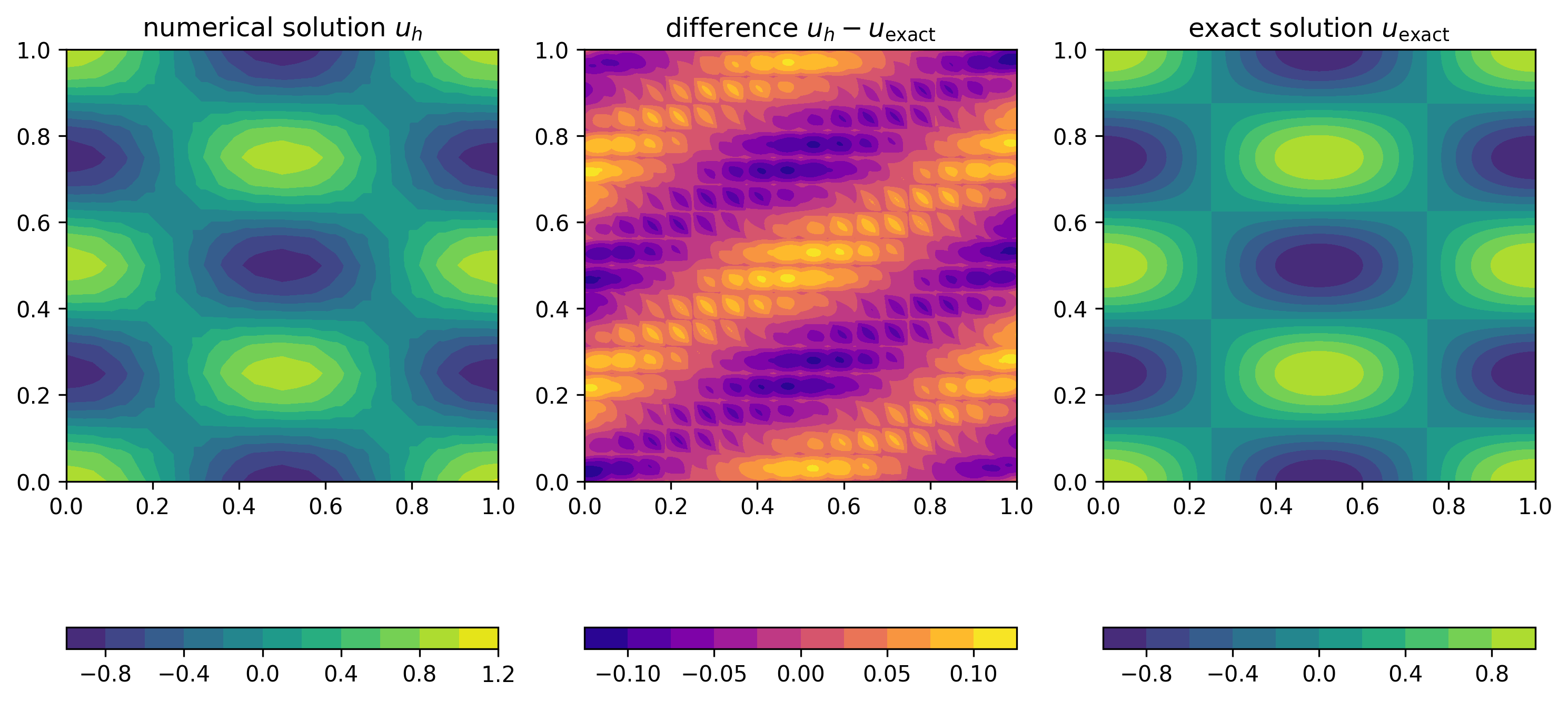
As Figure 19 demonstrates, using cubic elements on the same mesh improves the solution.

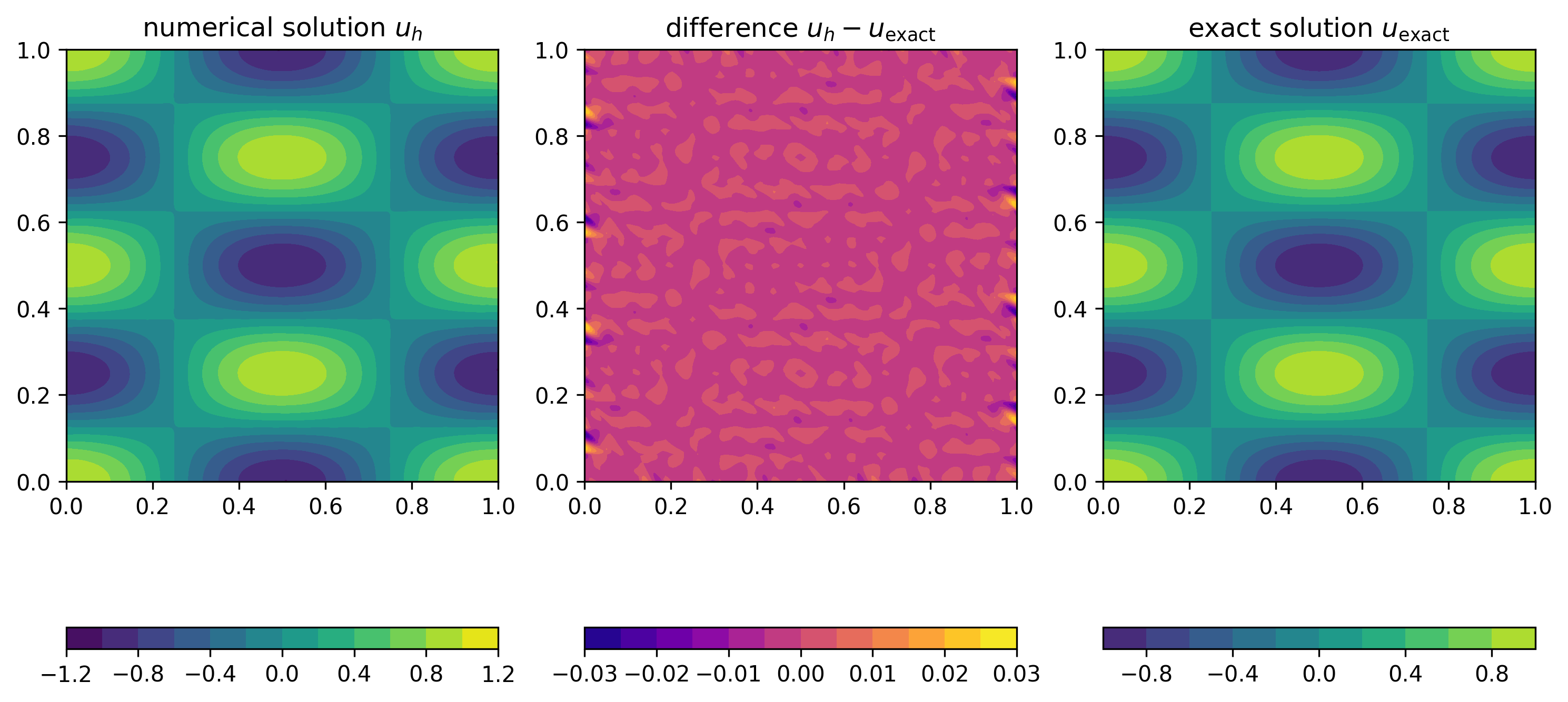
Figure 19: Visualisation of finite element solution and error for piecewise cubic finite elements

Performance

To obtain a more accurate solution we need to increase the resolution, which will make the computation more expensive. To expore this, let us now have a closer look at how the runtime of the code changes with the problem size. Usually, most of the time is spent executing a small number of lines.

To measure the time spent in some part of the code we use the measure_time(label) decorator defined in fem/utilities.py. This can be used as follows

with measure_time("some_code"):
    # Code to measure

Have a look at driver.py where the time spent in the following components is measured:

Assembly of right hand side $\boldsymbol{b}^{(h)}$ with assemble_rhs()
Assembly of stiffness matrix $A^{(h)}$ with assemble_lhs()
Solution of the linear system $A^{(h)}\boldsymbol{u}^{(h)} = \boldsymbol{b}^{(h)}$ with np.linalg.solve()

Figure 20 (left) shows the time spent in these parts of the code for increasing problem size. To confirm that the increase in resolution results in a more accurate solution, we also show the decrease of the $L_2$ error in Figure 20 (right). In both plots the horizontal axis shows the total number of unknowns $n_{\text{dof}}$, which is proportional to $h^{-2}$, the square of the inverse grid spacing.

Figure 20: Runtime (left) and L_2 error (right) — Figure 20: Runtime (left) and $L_2$ error (right)

The right plot confirms that the $L_2$ error decreases in proportion to $h^2\propto n_{\text{dof}}^{-1}$. As can be seen from the left plot, for larger problems, the time spent in the assembly of the stiffness matrix and right hand side increases in direct proportion to the problem size $n_{\text{dof}}$. This is not very surprising since (for fixed polynomial degree) the amount of work required in each grid cell remains approximately constant while the number of grid cells is directly proportional to the number of unknowns $n_{\text{dof}}$.

In contrast, the time spent in the solution of the linear system $A^{(h)}\boldsymbol{u}^{(h)}=\boldsymbol{b}^{(h)}$ grows much more rapidly with $\propto n_{\text{dof}}^3$: solving a problem with $16641$ unknowns takes around $48$ seconds. If we want to reduce the $L_2$ error to $10^{-5}$ we would need to solve a problem with $1.3\cdot 10^6$ (=1.3 million) unknowns. Extrapolating the measured time, solving a problem of this size would take $264$ days!

In the next section we will discuss methods for overcoming this difficulty. For this, we will need to go back to the sparse matrix storage format in PETSc. But before doing this, let us try to understand why the solve time increases with the third power of the problem size.

Complexity analysis

Let us assume that we want to solve a linear system $A\boldsymbol{u}=\boldsymbol{b}$ where $\boldsymbol{u}, \boldsymbol{b}\in\mathbb{R}^n$ and $A$ is a $n\times n$ matrix. The numpy.linalg.solve() method uses Gaussian elimination for this (in fact, it uses a slightly different method called $LU$ factorisation, but the central idea is the same). To illustrate this method, consider the following $5\times 5$ system (the rationale behind the colouring will become evident below):

\[ \underbrace{ \begin{pmatrix} \textcolor{red}{1.096} & \textcolor{black}{0.3391} & \textcolor{black}{0.0632} & \textcolor{black}{0.0555} & \textcolor{black}{0.2176}\\ \textcolor{green}{0.3687} & \textcolor{blue}{1.311} & \textcolor{blue}{0.0862} & \textcolor{blue}{0.3232} & \textcolor{blue}{0.0849}\\ \textcolor{green}{0.2743} & \textcolor{blue}{0.2277} & \textcolor{blue}{1.15} & \textcolor{blue}{0.0511} & \textcolor{blue}{0.2343}\\ \textcolor{green}{0.1019} & \textcolor{blue}{0.0976} & \textcolor{blue}{0.0082} & \textcolor{blue}{1.285} & \textcolor{blue}{0.3212}\\ \textcolor{green}{0.3629} & \textcolor{blue}{0.2885} & \textcolor{blue}{0.012} & \textcolor{blue}{0.1747} & \textcolor{blue}{1.145} \end{pmatrix}}_{=A} \underbrace{\begin{pmatrix} u_0 \\ u_1 \\ u_2 \\ u_3 \\ u_4 \end{pmatrix}}_{=\boldsymbol{u}} = \underbrace{ \begin{pmatrix} \textcolor{black}{0.23}\\ \textcolor{blue}{0.51}\\ \textcolor{blue}{0.29}\\ \textcolor{blue}{0.82}\\ \textcolor{blue}{0.98} \end{pmatrix}}_{=\boldsymbol{b}} \]

First, the system is slowly transformed into an equivalent upper triangular system as follows:

Reduction to upper triangular system

In the first step, we eliminate all entries below the diagonal in the first row (as before, we start counting at zero to be consistent with Python’s numbering convention), i.e. the entries shown in green in the equation above. For this, we go through all matrix rows $i=1,2,\dots,n-1$ and add the multiple $-\textcolor{green}{A_{i0}}/\textcolor{red}{A_{00}}$ of the first matrix row to row $i$, i.e. $\textcolor{blue}{A_{ij}} \mapsto \textcolor{blue}{A_{ij}} - \textcolor{green}A_{i0}/\textcolor{red}{A_{00}}\cdot A_{0j}$ for $j=0,1,2,\dots,n-1$. Here $\textcolor{red}{A_{00}}$, shown in red in the equation above, is known as the pivot. Observe that we do not have to do this calculation for the first column size the result will be zero by construction. At the same time, we need to modify the right hand side vector $\boldsymbol{b}$: all entries $b_i$ with $i=1,2,\dots,n-1$ get replaced by $b_i \mapsto b_i - \textcolor{green}{A_{i0}}/\textcolor{red}{A_{00}}\cdot b_0$. The following equation shows the matrix and right hand side vector after this transformation:

\[ \begin{aligned} A &= \begin{pmatrix} 1.096 & 0.3391 & 0.0632 & 0.0555 & 0.2176\\ \textcolor{lightgray}{0} & \textcolor{red}{1.197} & \textcolor{black}{0.06495} & \textcolor{black}{0.3045} & \textcolor{black}{0.01172}\\ \textcolor{lightgray}{0} & \textcolor{green}{0.1429} & \textcolor{blue}{1.134} & \textcolor{blue}{0.03721} & \textcolor{blue}{0.1799}\\ \textcolor{lightgray}{0} & \textcolor{green}{0.06608} & \textcolor{blue}{0.002326} & \textcolor{blue}{1.28} & \textcolor{blue}{0.301}\\ \textcolor{lightgray}{0} & \textcolor{green}{0.1763} & \textcolor{blue}{-0.008921} & \textcolor{blue}{0.1563} & \textcolor{blue}{1.073} \end{pmatrix} & b &= \begin{pmatrix} 0.23\\ \textcolor{black}{0.4326}\\ \textcolor{blue}{0.2325}\\ \textcolor{blue}{0.7986}\\ \textcolor{blue}{0.9039} \end{pmatrix} \end{aligned} \]

Note that the first row remains unchanged. To implement this transformation we need to carry out the following operations for each of the $n-1$ rows $i=1,2,\dots,n-1$:

compute $\rho_i = -A_{i0}/A_{00}$ $\Rightarrow$ $\boldsymbol{1}$ division
scale the first row by the factor $\rho_i$ and add the scaled first row to row $i$ $\Rightarrow$ $\boldsymbol{n-1}$ multiplications and $\boldsymbol{n-1}$ additions, since we can ignore the first entry which will be set to zero by construction
update $b_i \gets b_i - \rho_i \cdot b_0$ $\Rightarrow$ $\boldsymbol{1}$ multiplication and $\boldsymbol{1}$ subtraction

Hence, the total number of operations for processing all $n-1$ rows is $(3+2(n-1))(n-1)$.

Next, we repeat the same procecure for the $(n-1)\times (n-1)$ matrix in the lower right corner to zero-out all entries below the diagonal in the second column:

\[ \begin{aligned} A &= \begin{pmatrix} 1.096 & 0.3391 & 0.0632 & 0.0555 & 0.2176\\ \textcolor{lightgray}{0} & 1.197 & 0.06495 & 0.3045 & 0.01172\\ \textcolor{lightgray}{0} & \textcolor{lightgray}{0} & \textcolor{red}{1.127} & \textcolor{black}{0.0008768} & \textcolor{black}{0.1785}\\ \textcolor{lightgray}{0} & \textcolor{lightgray}{0} & \textcolor{green}{-0.001259} & \textcolor{blue}{1.263} & \textcolor{blue}{0.3003}\\ \textcolor{lightgray}{0} & \textcolor{lightgray}{0} & \textcolor{green}{-0.01848} & \textcolor{blue}{0.1115} & \textcolor{blue}{1.071} \end{pmatrix} & b &= \begin{pmatrix} 0.23\\ 0.4326\\ \textcolor{black}{0.1808}\\ \textcolor{blue}{0.7747}\\ \textcolor{blue}{0.8402} \end{pmatrix} \end{aligned} \]

Observe that the first two rows are not modified. Iterating, we get in the same fashion:

\[ \begin{aligned} A &= \begin{pmatrix} 1.096 & 0.3391 & 0.0632 & 0.0555 & 0.2176\\ \textcolor{lightgray}{0} & 1.197 & 0.06495 & 0.3045 & 0.01172\\ \textcolor{lightgray}{0} & \textcolor{lightgray}{0} & 1.127 & 0.0008768 & 0.1785\\ \textcolor{lightgray}{0} & \textcolor{lightgray}{0} & \textcolor{lightgray}{0} & \textcolor{red}{1.263} & \textcolor{black}{0.3005}\\ \textcolor{lightgray}{0} & \textcolor{lightgray}{0} & \textcolor{lightgray}{0} & \textcolor{green}{0.1115} & \textcolor{blue}{1.074} \end{pmatrix} & b &= \begin{pmatrix} 0.23\\ 0.4326\\ 0.1808\\ \textcolor{black}{0.7749}\\ \textcolor{blue}{0.8431} \end{pmatrix} \end{aligned} \]

and finally

\[ \begin{aligned} A &= \begin{pmatrix} 1.096 & 0.3391 & 0.0632 & 0.0555 & 0.2176\\ \textcolor{lightgray}{0} & 1.197 & 0.06495 & 0.3045 & 0.01172\\ \textcolor{lightgray}{0} & \textcolor{lightgray}{0} & 1.127 & 0.0008768 & 0.1785\\ \textcolor{lightgray}{0} & \textcolor{lightgray}{0} & \textcolor{lightgray}{0} & 1.263 & 0.3005\\ \textcolor{lightgray}{0} & \textcolor{lightgray}{0} & \textcolor{lightgray}{0} & \textcolor{lightgray}{0} & 1.047 \end{pmatrix} & b &= \begin{pmatrix} 0.23\\ 0.4326\\ 0.1808\\ 0.7749\\ 0.7747 \end{pmatrix} \end{aligned} \]

Total computational cost

The number of operations to carry out this procedure is obtained by summing the number of operations for all $n-1$ steps:

\[ \begin{aligned} n_{\text{solve}}(n) &= (3+2(n-1))(n-1) + (3+2(n-2))(n-2) + \dots +(3+2\cdot 1)\cdot 1\\ &= \sum_{k=1}^{n-1} (3+2k)k\\ &= \frac{3}{2} n(n-1) + \frac{1}{3} n(n-1)(2n-1)\\ &= \frac{2}{3} n^3 + \mathcal{O}(n^2) \end{aligned} \]

Finally, we need to solve the upper triangular system that is obtained by following this algorithm. As can be shown (see exercise), the cost of this is $\mathcal{O}(n^2)$.

We conclude that the cost of the linear solve is $\frac{2}{3}n^3 + \mathcal{O}(n^2)$: for very large values of $n$ the cost will grow with the third power of the problem size, exactly as observed in Figure 20 (left).

Cost of floating point operations

Based on the discussion in the previous section and the data in Figure 20 (left), we can also work out the time $t_{\text{flop}}$ it takes to carry out a single floating point operation (FLOP). This is a useful exercise, since knowing this number will allow us to construct a simple performance model for predicting the runtime of any other given algorithm: if the algorithm requires $n_{\text{flop}}$ FLOPs, then the predicted runtime is

\[ T = n_{\text{flop}}\cdot t_{\text{flop}}. \]

In particular, the total time can be separated into the product of two factors:

the number of FLOPs $n_{\text{flop}}$ which depends on the algorithm, but is independent of the computer the code is run on and
the machine dependent time $t_{\text{flop}}$

Looking at the measured data, we observe that we measured $T_{\text{solve}}= 48.4\text{s}$ for $n=166411$. Since $n\gg 1$ we can ignore the $\mathcal{O}(n^2)$ terms in the expression for the number of flops and therefore:

\[ t_{\text{flop}} = \frac{T_{\text{solve}}}{n_{\text{solve}}} \approx \frac{48.4\text{s}}{\frac{2}{3}\cdot 16641^3} \approx 1.6\cdot 10^{-11}\text{s} \]

In other words, on the specific machine we can carry out

\[ R = t_{\text{flop}}^{-1} = 6.3\cdot 10^{10} \]

floating point operations per second. Obviously, this number will be machine dependent, but on modern computers it is usually in the same ballpark.

Solving sparse linear systems

To reduce the cost spent in solving the linear system $A^{(h)}\boldsymbol{u}^{(h)} = \boldsymbol{b}^{(h)}$ we will devise more efficient algorithms which are tailored to the particular structure of the problem. In particular, we will exploit the fact that the stiffness matrix $A^{(h)}$ of our finite element discretisation contains a lot of zero entries. Consider, for example, the $81\times 81$ matrix that is obtained for a piecewise linear discretisation on a $8\times 8$ grid (plots like this can be generated with matplotlib’s spy() function):

Figure 21: Spy plot of the stiffness matrix A^{(h)} — Figure 21: Spy plot of the stiffness matrix $A^{(h)}$

Of the $81\times 81 = 6561$ entries of this matrix, only $n_{\text{nz}}=497$ or $7.6\%$ are nonzero, which corresponds to an average number of around $\overline{n}_{\text{nz}} = 6.14$ nonzeros per row. For large $n$, the number of non-zeros per row will remain roughly the same, leading to an even poorer fill-ratio.

Clearly, it is very inefficient to store all these zero entries if only $\mathcal{O}(n)$ entries are in fact required to encode the data stored in the matrix. It is much more efficient to use the compressed sparse row (CSR) storage format introduced at the beginning of this course. For a matrix of size $n\times n$ with $n_{\text{nz}}$ nonzero entries this only requires the storage of $2n_{\text{nz}}+(n+1)$ numbers. If the number $n_{\text{nz}}/n\le C$ of non-zeros per row is bounded by some constant $C$ (as it is for the finite element stiffness matrices), then the total storage required is \[ 2n_{\text{nz}}+(n+1) = \left(2\frac{n_{\text{nz}}}{n}+1+\frac{1}{n}\right)\cdot n \le 2(C+1)\cdot n = \mathcal{O}(n) \] However, in addition to changing the matrix storage format we also need to adapt our solver.

Solving linear systems

The big advantage of using PETSc matrices and arrays is that this will give us access to a huge library of efficient solvers for sparse linear systems of the form $A\boldsymbol{u}=\boldsymbol{b}$. Let us just look at a simple example:

Consider the following $5\times 5$ matrix \[ A=\begin{pmatrix} 10.2 & 0.8 & \textcolor{lightgray}{0} & -2.1 & \textcolor{lightgray}{0}\\ 0.8 & 6.7 & \textcolor{lightgray}{0} & \textcolor{lightgray}{0} & \textcolor{lightgray}{0} \\ \textcolor{lightgray}{0} & \textcolor{lightgray}{0} & 6.4 & \textcolor{lightgray}{0} & \textcolor{lightgray}{0} \\ -2.1 & \textcolor{lightgray}{0} & \textcolor{lightgray}{0} & 7.2 & \textcolor{lightgray}{0} \\ \textcolor{lightgray}{0} & \textcolor{lightgray}{0} & \textcolor{lightgray}{0} & \textcolor{lightgray}{0} & 9.8 \end{pmatrix} \] which, in CSR format, corresponds to

row pointers $R = [0, 3, 5, 6, 8, 9]$
column indices $J = [0, 1, 3, 0, 1, 2, 0, 3, 4]$
values $V = [10.2, 0.8, -2.1, 0.8, 6.7, 6.4, -2.1, 7.2, 9.8]$

To create this matrix, we can proceed as follows:

row_start = [0, 3, 5, 6, 8, 9]
col_indices = [0, 1, 3, 0, 1, 2, 0, 3, 4]
values = [10.2, 0.8, -2.1, 0.8, 6.7, 6.4, -2.1, 7.2, 9.8]

A = PETSc.Mat().createAIJWithArrays(
    (5, 5),
    (
        row_start,
        col_indices,
        values,
    ),
)
A.assemble()

Observe that we created the matrix in one go by using createAIJWithArrays(), which gets passed the number of rows and columns and a tuple $(R,J,V)$. We can then solve the linear system $A\boldsymbol{u}=\boldsymbol{b}$ for given $\boldsymbol{b} = (8.1, 0, 9.3, -4.3, 5.2)^\top$ as follows by creating a KSP object, associating the matrix A with it and then calling the KSP’s solve method.

b = PETSc.Vec().createWithArray([8.1, 0, 9.3, -4.3, 5.2])
u = PETSc.Vec().createSeq(b.size)

ksp = PETSc.KSP().create()
ksp.setOperators(A)
ksp.solve(b, u)

Next, let us look in more detail at what the ksp.solve() method actually does.

Solvers and Preconditioners

Although PETSc also supports direct solvers such as Gaussian elimination (which we used above), the design philosophy of the library assumes that all solvers are iterative methods. This means that to solve problems of the form $A\boldsymbol{u}=\boldsymbol{b}$ we start from some initial guess, $\boldsymbol{u}^{(0)}$. Based on this, the solution is updated iteratively as $\boldsymbol{u}^{(k)}\mapsto \boldsymbol{u}^{(k+1)}$ such that (hopefully) $\boldsymbol{u}^{(k)}$ converges to the true solution $\boldsymbol{u}$. Direct solvers can be considered as a special case in which this iteration converges in a single step.

At this point it is worth remembering that (in addition to possible modelling errors) the finite element method has introduced a discretisation error. This implies that there is little point in solving the equation $A^{(h)}\boldsymbol{u}^{(h)}=\boldsymbol{b}^{(h)}$ exactly, it is usally sufficient to iterate until we have a good approximate solution which differs from the exact solution by no more than the discretisation error. This can lead to significant savings in runtime.

PETSc solver architecture

PETSc solvers are separated into two components:

an iterative solver or KSP object which describes how to perform the update $\boldsymbol{u}^{(k)}\mapsto \boldsymbol{u}^{(k+1)}$
a preconditioner or PC object which accelerates the iteration

To motivate this architecture and explain what a preconditioner is, let us consider a very simple iterative method. For this, we multiply the linear equation $A\boldsymbol{u}=\boldsymbol{b}$ by a matrix $P^{-1}$ to obtain the equivalent system

\[ P^{-1} A \boldsymbol{u} = P^{-1} \boldsymbol{b} \]

The matrix $P$, which we assume to be full rank and invertible, is the preconditioner. More precisely, in PETSc a PC object provides a way of inverting $P$, i.e. solving $P\boldsymbol{z}=\boldsymbol{r}$ for a given vector $\boldsymbol{r}$. In principle, we could choose any matrix such as $P=\mathbb{I}$ (the identity matrix) or $P=D$ (the diagonal of $A$). A good preconditioner has two properties:

It should be “close” to $A$, i.e. $P\approx A$ (in some sense which can be made mathematically rigorous)
Multiplication by $P^{-1}$ should be inexpensive, i.e. solving the linear system $P\boldsymbol{z}=\boldsymbol{r}$ for a given vector $\boldsymbol{r}$ should be cheap.

Naturally, these requirements often contradict each other and a compromise has to be found. The construction of a good preconditioner is an art in itself and the topic of active research.

Richardson iteration with Jacobi preconditioner

As an example, we now construct a very simple iterative procedure. Assume that we know the approximate solution $\boldsymbol{u}^{(k)}$. If we knew the error $\boldsymbol{e}^{(k)} := \boldsymbol{u}-\boldsymbol{u}^{(k)}$ (where $\boldsymbol{u}$ is the exact solution of $A\boldsymbol{u}=\boldsymbol{b}$), it would be possible to compute the solution by simply adding $\boldsymbol{e}^{(k)}$ to $\boldsymbol{u}^{(k)}$ since $\boldsymbol{u}^{(k)} + \boldsymbol{e}^{(k)} = \boldsymbol{u}$. Unfortunately, this is not possible since knowledge of $\boldsymbol{e}^{(k)}$ would require knowledge of the exact solution which we are trying to find in the first place! Instead, let us try to construct an approximation $\boldsymbol{z}^{(k)}$ to the true error, namely \[ \boldsymbol{z}^{(k)} = P^{-1} A \boldsymbol{e}^{(k)} \] If $P\approx A$, this will be a good approximation. Interestingly we can compute $\boldsymbol{z}^{(k)}$ without knowledge of $\boldsymbol{u}$ since \[ \begin{aligned} \boldsymbol{z}^{(k)} &= P^{-1} A (\boldsymbol{u}-\boldsymbol{u}^{(k)})\\ &= P^{-1}(A\boldsymbol{u}-A\boldsymbol{u}^{(k)})\\ &= P^{-1}(\boldsymbol{b}-A\boldsymbol{u}^{(k)}) \end{aligned} \] The quantity $\boldsymbol{z}^{(k)}$ is also known as the preconditioned residual, since the residual $\boldsymbol{b}-A\boldsymbol{u}^{(k)}$ itself measures by how much the approximate solution violates the equation $A\boldsymbol{u}=\boldsymbol{b}$.

This leads to the so-called preconditioned Richardson iteration: starting from some initial guess $\boldsymbol{u}^{(0)}$ (which could for example be chosen to be $\boldsymbol{u}^{(0)}=0$) update the approximate solution $\boldsymbol{u}^{(k)}\rightarrow \mapsto{u}^{(k+1)}$ accroding to the rule \[ \begin{aligned} \boldsymbol{u}^{(k+1)} &= \boldsymbol{u}^{(k)} + \boldsymbol{z}^{(k)}\\ &= \boldsymbol{u}^{(k)} + P^{-1}(\boldsymbol{b}-A\boldsymbol{u}^{(k)}) \end{aligned} \] This can be written as follows:

Algorithm: preconditioned Richardson iteration

Pick some initial guess $\boldsymbol{u}^{(0)}$
for $k=0,1,\dots,k_{\text{max}}-1$ do
$~~~~$ Compute the residual $\boldsymbol{r}^{(k)} = \boldsymbol{b} - A\boldsymbol{u}^{(k)}$
$~~~~$ Solve $P\boldsymbol{z}^{(k)} = \boldsymbol{r}^{(k)}$ for the preconditioned residual $\boldsymbol{z}^{(k)}$
$~~~~$ Test for convergence, for example by checking whether $\|\boldsymbol{z}^{(k)}\|\le \epsilon$ for some tolerance $\epsilon$
$~~~~$ Update $\boldsymbol{u}^{(k+1)} = \boldsymbol{u}^{(k)} + \boldsymbol{z}^{(k)}$
end for

It can be shown that \[ \boldsymbol{e}^{(k+1)} = \left(\mathbb{I} - P^{-1} A\right)\boldsymbol{e}^{(k)}. \] Hence, if the spectral radius of $\mathbb{I} - P^{-1} A$ is smaller than $1$, the iteration will converge to the true solution.

Note in particular that if we set $P=A$, the iteration converges in a single step.

One possible preconditioner is the diagonal $D$ of $A$, i.e. \[ D_{ij} = \begin{cases} A_{ii} & \text{if $i=j$}\\ 0 & \text{otherwise} \end{cases} \] This matrix is very simple to invert: to solve $P\boldsymbol{z}=\boldsymbol{r}$ we can compute $z_i = r_i/A_{ii}$ for all $i=0,1,2,\dots,n-1$. The choice $P=D$ is also known as the Jacobi preconditioner.

PETSc options

To use a particular solver/preconditioner combination in PETSc, we can specify solver options via the command line. For this, we need to add the following at the beginning of our Python script:

import sys
import petsc4py

petsc4py.init(sys.argv)

This will ensure than any options passed to the script are parsed by PETSc. Then, when setting up the KSP object, we instruct PETSc to use the command line options with

ksp.setFromOptions()

For example, to use the Richardson iteration with Jacobi preconditioner, we would call our script like this:

python script.py -ksp_type richardson -pc_type jacobi

To monitor convergence, we can add the option -ksp_monitor, which will print out the norm $\|\boldsymbol{z}^{(k)}\|$ of the (preconditioned) residual at each iteration. The iteration will stop once the residual norm has been reduced by a factor of at least $\epsilon$, i.e. $\|\boldsymbol{z}^{(k)}\|/\|\boldsymbol{z}^{(0)}\|<\epsilon$. This tolerance can be controlled by -ksp_rtol epsilon. It is also possible to set an absolute convergence criterion $\|\boldsymbol{z}^{(k)}\|<\epsilon_{\text{abs}}$ with -ksp_atol epsilon_abs; in fact the iteration will stop once $\|\boldsymbol{z}^{(k)}\|<\operatorname{max}\{\epsilon\cdot \|\boldsymbol{z}^{(0)}\|,\epsilon_{\operatorname{abs}}\}$. The default values are $\epsilon=10^{-5}$, $\epsilon_{\text{abs}}=10^{-50}$.

Furthermore, we can tell PETSc to print information on the solver to some file ksp_view.txt with -ksp_view :ksp_view.txt. So, in summary to solve to a relative tolerance of $\epsilon=10^{-9}$ with the Jacobi-preconditioned Richardson iteration we would call:

python script.py -ksp_type richardson -pc_type jacobi -ksp_monitor -ksp_rtol 1.0E-9 -ksp_view :ksp_view.txt

The output looks like this:

  0 KSP Residual norm 1.838591537060e+00
  1 KSP Residual norm 2.788478455780e-01
  2 KSP Residual norm 6.738101826929e-02
  3 KSP Residual norm 1.935593309132e-02
  4 KSP Residual norm 4.677183280874e-03
  5 KSP Residual norm 1.343571957886e-03
  6 KSP Residual norm 3.246618113646e-04
  7 KSP Residual norm 9.326264962292e-05
  8 KSP Residual norm 2.253606186213e-05
  9 KSP Residual norm 6.473729794262e-06
 10 KSP Residual norm 1.564317287780e-06
 11 KSP Residual norm 4.493672185454e-07
 12 KSP Residual norm 1.085854572401e-07
 13 KSP Residual norm 3.119235806950e-08
 14 KSP Residual norm 7.537346563530e-09
 15 KSP Residual norm 2.165184982094e-09
 16 KSP Residual norm 5.231969233880e-10

and we can inspect the file ksp_view.txt to double check that the solver options have been set correctly:

At the beginning, the file ksp_view.txt lists details on the KSP Object, which describes the iterative solver, including the used tolerances $\epsilon$, $\epsilon_{\text{abs}}$:

KSP Object: 1 MPI process
  type: richardson
    damping factor=1.
  maximum iterations=10000, initial guess is zero
  tolerances: relative=1e-09, absolute=1e-50, divergence=10000.
  left preconditioning
  using PRECONDITIONED norm type for convergence test

This is followed by details on the PC Object, which describes the preconditioner:

PC Object: 1 MPI process
  type: jacobi
    type DIAGONAL
  linear system matrix = precond matrix:
  Mat Object: 1 MPI process
    type: seqdense
    rows=5, cols=5
    total: nonzeros=25, allocated nonzeros=25
    total number of mallocs used during MatSetValues calls=0

It is a good idea to double check the log_view output since it is very easy to inadvertedly use incorrect solver settings. The PETSc documentation contains further details on the available solvers and preconditioners. For example, the Richardson iteration is described under KSPRICHARDSON and the Jacobi preconditioner is described under PCJACOBI. Can you work out how to use the additional damping factor scale? Does choosing a value for this parameter which differs from the default of $1.0$ improve convergence?

Direct solvers

PETSc also supports direct solvers, which are implemented as preconditioners. For example, to use Gaussian elimination, we would set -pc_type lu. In this case, PETSc computes the factorisation $P=A=LU$, where $L$ and $U$ and lower- and upper-triangular matrices. Knowing $L$ and $U$ we can solve $A\boldsymbol{z}=LU\boldsymbol{z}=\boldsymbol{r}$ by solving $L\boldsymbol{z}'=\boldsymbol{r}$ and then $U\boldsymbol{z}=\boldsymbol{z}'$. In this case, the iterative solver will converge in a single iteration:

  0 KSP Residual norm 1.752245775437e+00
  1 KSP Residual norm 9.063045098981e-17

We can request that PETSc only applies the preconditioner, i.e. computes $\boldsymbol{u}^{(1)} = P^{-1}\boldsymbol{b}$ directly, which is sensible if the preconditioner is a direct solver. For this we set -ksp_type preonly. Be careful with using this option: if the preconditioner is not a direct solver, the iteration will simply stop after one iteration and return an incorrect result. For example, -ksp_type preonly -pc_type richardson will print out

  0 KSP Residual norm 1.405809375413e+01
  1 KSP Residual norm 2.181187602316e+00

and it is up to the user to recognise that the computed solution does in fact not solve $A\boldsymbol{u}=\boldsymbol{b}$.

Conjugate Gradient method

The (preconditioned) Richardson iteration is not very efficient. A better alternative for symmetric positive definite (SPD) $A$ is the Conjugate Gradient algorithm, which is given as follows:

Algorithm: Conjugate Gradient method 1. Set $\boldsymbol{r}^{(0)}\gets \boldsymbol{b} - A\boldsymbol{u}^{(0)}$ 2. Solve $P\boldsymbol{z}^{(0)} = \boldsymbol{r}^{(0)}$ 3. Set $\boldsymbol{p}^{(0)}\gets \boldsymbol{z}^{(0)}$ 4. for $k=1,2,\dots,k_{\text{max}}$ do 5. $~~~~$ Compute $\alpha_{k-1} = \boldsymbol{z}^{(k-1)\top} \boldsymbol{r}^{(k-1)}/\boldsymbol{p}^{(k-1)\top} A\boldsymbol{p}^{(k-1)}$ 6. $~~~~$ Set $\boldsymbol{u}^{(k)} \gets \boldsymbol{u}^{(k-1)} + \alpha_{k-1} \boldsymbol{p}^{(k-1)}$ 7. $~~~~$ Set $\boldsymbol{r}^{(k)} \gets \boldsymbol{r}^{(k-1)} - \alpha_k A \boldsymbol{p}^{(k-1)}$ 8. $~~~~$ Check convergence 9. $~~~~$ Solve $P\boldsymbol{z}^{(k)}=\boldsymbol{r}^{(k)}$ for $\boldsymbol{z}^{(k)}$ 10. $~~~~$ Compute $\beta_k = \boldsymbol{z}^{(k)\top}\boldsymbol{r}^{(k)}/\boldsymbol{z}^{(k-1)\top}\boldsymbol{r}^{(k-1)}$ 11. $~~~~$ Set $\boldsymbol{p}^{(k)} \gets \boldsymbol{z}^{(k)} + \beta_k \boldsymbol{p}^{(k-1)}$ 12. end do

Crucially, the fundamental operations that are required are very similar to those in the Richardson iteration

multiplication of a vector $\boldsymbol{x}$ with the matrix $A$ to compute $\boldsymbol{y}=A\boldsymbol{x}$
addition and scaling of vectors: $\boldsymbol{z} = \alpha \boldsymbol{x}+\beta \boldsymbol{y}$ for $\alpha,\beta\in\mathbb{R}$
dot-products of vectors: $\boldsymbol{x}^\top\boldsymbol{y}=\sum_{i=0}^{n-1} x_i y_i$
Preconditioner applications: solve $P\boldsymbol{z}=\boldsymbol{r}$ for $\boldsymbol{z}$

In PETSc, the Conjugate Gradient method can be invoked with -ksp_type cg. If we repeat the numerical experiment above with

python script.py -ksp_type cg -pc_type jacobi -ksp_monitor -ksp_rtol 1.0E-9 -ksp_view :ksp_view.txt

we get the following output:

  0 KSP Residual norm 1.838591537060e+00
  1 KSP Residual norm 2.299841486091e-01
  2 KSP Residual norm 2.631059255681e-02
  3 KSP Residual norm 2.056954907970e-17

i.e. the solver converges in substantially fewer iterations than the Richardson iteration. We will compare different solver and preconditioner settings for the finite element stiffness matrix below.

Other Krylov subspace methods

The Conjugate Gradient (CG) algorithm is an example of a so-called Krylov subspace method. While the CG iteration only works for SPD matrices, there are other Krylov subspace methods that can be used for more general matrices. The most important one is the Generalised Minimal Residual (GMRES) method, which can be invoked with -ksp_type gmres. The details are not relevant for this course, but it should be pointed out that GMRES only requires the same fundamental linear algebra operations as CG and the Richardson iteration.

Having introduced PETSc solvers, let us now go back to the solution of the linear problem $A^{(h)}\boldsymbol{u}^{(h)}=\boldsymbol{b}^{(h)}$ that arises in the finite element discretisation.

Assembly of sparse stiffness matrix

To assemble the stiffness matrix $A^{(h)}$ in CSR format, we first need to work out the sparsity structure, i.e. build the lists containing the column indices $J$ and row-pointers $R$.

Sparsity structure

For this observe that for the row of $A^{(h)}$ with index $\ell_{\text{global}}$ we need to find the set of indices $\mathcal{J}_{\ell_{\text{global}}}$ such that $A^{(h)}_{\ell_{\text{global}},k_{\text{global}}} \neq 0$ for all $k_{\text{global}}\in \mathcal{J}_{\ell_{\text{global}}}$. To construct this set, observe that all unknowns associated with a given cell with index $\alpha$ couple to each other, i.e. $A^{(h)}_{\ell_{\text{global}},k_{\text{global}}} \neq 0$ for all $\ell_{\text{global}},k_{\text{global}}\in \mathcal{L}^{(K)} = \{\ell_{\text{global}}(\alpha,\ell)\;\text{for}\;\ell=0,1,\dots,\nu-1\}$ the set of global indices of unknowns associated with cell $K$. We can therefore construct the sets $\mathcal{J}_{\ell_{\text{global}}}$ by visiting all cells of the mesh and inserting the correct indices. Once we have done this, we use the information in $\mathcal{J}_{\ell_{\text{global}}}$ to construct the column index array $J$ and the row-pointer array $R$ as shown in the following procedure:

Algorithm: create sparsity structure

Set $\mathcal{J}_{\ell_{\text{global}}} = \emptyset$ for all $\ell_{\text{global}}=0,1,\dots,n_{\text{dof}}-1$
for all cells $K$ with index $\alpha$
$~~~~$ Set $\mathcal{L}^{(K)} = \{\ell_{\text{global}}(\alpha,\ell)\;\text{for}\;\ell=0,1,\dots,\nu-1\}$, the set of global indices of dofs associated with cell $K$
$~~~~$ for all $\ell_{\text{global}}\in \mathcal{L}^{(K)}$ do
$~~~~~~~~$ Update $\mathcal{J}_{\ell_{\text{global}}} \gets \mathcal{J}_{\ell_{\text{global}}} \cup \mathcal{L}^{(K)}$
$~~~~$ end do
end do
Initialise row pointer array $R = [0,0,\dots,0]\in \mathbb{R}^{n+1}$
Initialise column index array $J = []$
for $\ell_{\text{global}}=0,1,\dots,n_{\text{dof}}-1$ do
$~~~~$ Append $\mathcal{J}_{\ell_{\text{global}}}$ to $J$
$~~~~$ Set $R_{\ell_{\text{global}}+1} = R_{\ell_{\text{global}}} +\left|\mathcal{J}_{\ell_{\text{global}}}\right|$
end do

In fem/assembly.py this is implemented as the function sparsity_lhs(fs) which gets passed an instance fs of the FunctionSpace class and returns the arrays $J$ and $R$.

CSR matrix assembly in PETSc

When using PETSc, the stiffness matrix $A^{(h)}$ can be assembled as follows. First, before iterating over the mesh, we need to work out the sparsity structure and construct the row-pointers row_start and column indices col_indices with the above algorithm. Assuming that the function space object is fs, this can be done with the method sparsity_lhs(fs). We also need to construct the stiffness_matrix as a PETSc.Mat() object in CSR format which is initialised with the row_start and col_indices arrays returned by sparsity_lhs(fs):

row_start, col_indices = sparsity_lhs(fs)
stiffness_matrix = PETSc.Mat()
stiffness_matrix.createAIJ((fs.ndof, fs.ndof), csr=(row_start, col_indices))

Recall that previously we inserted the cell-local matrix local_matrix into the correct position in the global stiffness_matrix with

stiffness_matrix[np.ix_(j_g, j_g)] += local_matrix

where stiffness_matrix is a dense numpy array and j_g is the list of global dof-indices associated with a particular cell $K$. When using PETSc this needs to be replaced by

stiffness_matrix.setValues(j_g, j_g, local_matrix, addv=True)

where the addv=True parameter ensures that the matrix elements are incremented (compare to the += in the native assembly).

Finally, after iterating over the mesh, we need to instruct PETSc to assemble the matrix with

stiffness_matrix.assemble()

The code for assembly of the stiffness matrix can be found in fem/assembly.py. The function assemble_lhs_sparse(fs, quad, kappa, omega) gets passed an instance fs of the FunctionSpace class, a quadrature rule and the constants $\kappa$, $\omega$ that define the PDE. It returns the assembled stiffness matrix $A^{(h)}$ as a PETSc CSR matrix.

The full code for solving the finite element problem with PETSc matrices and solvers can be found in driver_sparse.py, which should be compared to the non-PETSc version in driver.py.

To run the code for a specific solver and preconditioner we again pass PETSc solver options via the command line, for example:

python driver_sparse.py -ksp_type richardson -pc_type jacobi -ksp_rtol 1.0E-6 -ksp_monitor -ksp_view :ksp_view.txt

Performance analysis

Let us try to understand the performance of the iterative solver algorithm. We start with the simplest version, namely the Richardson iteration with Jacobi preconditioner. Recall that this requires the following operations:

Computation of the residual $\boldsymbol{r} = \boldsymbol{b} - A\boldsymbol{u}$
Application of the diagonal preconditioner $\boldsymbol{z} = D^{-1} \boldsymbol{r}$
Update of the solution vector $\boldsymbol{u}\mapsto \boldsymbol{u} + \boldsymbol{z}$

We count the number of operations as follows: firstly, when computing the residual $\boldsymbol{r} = \boldsymbol{b} - A\boldsymbol{u}$ we need to apply one subtraction and one multiplication for each non-zero matrix element $A_{ij}$ when computing $r_i \mapsto r_i - A_{ij} u_j$ (applying the matrix, i.e. computing $\boldsymbol{v} = A\boldsymbol{u}$ requires the same number of operations). The application of the preconditioner $\boldsymbol{z} = D^{-1} \boldsymbol{r}$ requires one division per vector element and finally the update $\boldsymbol{u}\mapsto \boldsymbol{u} + \boldsymbol{z}$ of the solution requires one addition for each vector element. Hence, the total number of floating point operations for a single Richardson update with Jacobi preconditioner requires

\[ N_{\text{Ric+Jac}} = 2n_{\text{nz}} + 2n \]

floating point operations (FLOPs). Assume, for example, that $n=16641$ and $n_{\text{nz}}=115457$ (piecewise linear elements, rectange mesh with nref=7), then $N_{\text{Ric+Jac}} = 264196$. Recall that $t_{\text{flop}} = 1.6\cdot 10^{-11}\text{s}$, so we would expect that a single Richardson+Jacobi iteration takes around

\[ \begin{aligned} T_{\text{Ric+Jac}} &= (2n_{\text{nz}} + 2n)t_{\text{flop}}\\ &= 264196 \cdot 1.6\cdot 10^{-11}\text{s}\\ &= 4.2\mu\text{s} \end{aligned} \]

However, in fact we measure $T_{\text{Ric+Jac}} = 85.6\mu\text{s}$, i.e. a number which is more than an order of magnitude larger than expected!

Instead of using the measure_time decorator, we could also pass the option -log_view to PETSc to get more information on the performance of individual components of the code. For this, we run the code with

python driver_sparse.py -ksp_type richardson -pc_type jacobi -ksp_rtol 1.0E-6 -ksp_monitor -ksp_view :ksp_view.txt -log_view :log_view.txt

and inspect the generated file log_view.txt. The matrix-vector product MatMult is executed $37049$ times, and in total $2.734\text{s}$ are spent in this part of the code. This implies $73.7\mu\text{s}$ per matrix-vector product, compared to the theoretical prediction $T_{\text{MatMult}} = 2n_{\text{nz}}t_{\text{flop}}=2\cdot 115457\cdot 1.6\cdot 10^{-11}\text{s} = 3.7\mu\text{s}$. Again, our performance model is off by more than order of magnitude!

Memory references

The reason for the mismatch between the model and the measurements is that reading data from memory and writing it back is not free: To compute the matrix-vector product $\boldsymbol{v} = A\boldsymbol{u}$ we need to read the vector $\boldsymbol{u}$, write back the vector $\boldsymbol{v}$ and read the arrays $I$, $R$ and $V$ which represent the matrix $A$ in CSR format. The total amount of data transferred between the CPU and main memory is:

Read $\boldsymbol{u}$: $n$ double precision (64 bit) floating point numbers
Write $\boldsymbol{v}$: $n$ double precision floating point numbers
Read value array $V$: $n_{\text{nz}}$ double precision numbers
Read row pointer array $I$: $n+1$ integer numbers (32 bit each)
Read column index array $J$: $n_{\text{nz}}$ integer numbers (32 bit each)

The total amount of transferred memory is therefore

\[ M_{\text{MatMult}} = \frac{3}{2} n_{\text{nz} + }\frac{5}{2} n + \frac{1}{2} \]

double precision numbers. Assuming that it takes $t_{\text{mem}}$ to transfer a single double precision number, this implies that the total time to execute the matrix-vector product is:

\[ \begin{aligned} T_{\text{MatMult}} &= M_{\text{MatMult}} t_{\text{mem}} + N_{\text{MatMult}} t_{\text{flop}}\\ &= \left(\frac{3}{2} n_{\text{nz} + }\frac{5}{2} n + \frac{1}{2}\right) t_{\text{mem}} + 2(n_{\text{nz}}+n)t_{\text{flop}} \end{aligned} \]

Plugging in the measured value of $T_{\text{MatMult}}=73.7\mu\text{s}$ and solving for the unknown $t_{\text{mem}}$ we find

\[ t_{\text{mem}} = 3.2\cdot 10^{-10} \text{s}= 20\times t_{\text{flop}}. \]

From this we conclude that it is about an order of magnitude more expensive to transfer a double precision variable from memory than doing the actual computation!

We can also define the memory bandwidth, i.e. the number of double precision numbers of bytes that can be transferred per second as

\[ BW = t_{\text{mem}}^{-1} = 3.12 \cdot 10^9 \text{double}/\text{s} = 2.5\cdot 10^{10} \text{byte}/\text{s} \]

Why did this not matter for the Gaussian elimination solver? The reason is that the number of floating point operations is much larger than the number of memory references in this case: recall the that number of operations to solve a system with Gaussian elimination is $\frac{2}{3}n^3 + \mathcal{O}(n^2)$, where we can neglect the $\mathcal{O}(n^2)$ correction for $n\gg 1$. In addition we need to read the matrix ($n^2$ double precision numbers), read the vector $\boldsymbol{u}$ ($n$ double precision numbers) and write $\boldsymbol{v}$ (also $n$ double precision numbers). Including the cost of memory transfers we find:

\[ \begin{aligned} T_{\text{Gauss}} &= \left(n^2 + 2n\right)t_{\text{mem}} + \frac{2}{3}n^3 t_{\text{flop}}\\ &= \frac{2}{3}n^3 t_{\text{flop}}\left(1 + \frac{n^2 + 2n}{\frac{2}{3}n^3}\frac{t_{\text{mem}}}{t_{\text{flop}}} \right)\\ &\approx \frac{2}{3}n^3 t_{\text{flop}}\left(1 + \frac{2}{3n}\frac{t_{\text{mem}}}{t_{\text{flop}}} \right) \end{aligned} \]

For $n\gg \frac{t_{\text{mem}}}{t_{\text{flop}}}\approx 20$ we can safely ignore the second term in the bracket and recover the previously used performance model.

We also say that Gaussian elemination if FLOP-bound whereas the CSR matrix-vector product and hence the iterative solve with the Richardson+Jacobi iteration is memory bandwidth-bound.

Roofline model

More generally, consider an algorithm with $N$ FLOPs and $M$ (double precision) memory references and define the arithmetic intensity

\[ q := \frac{N}{M}, \]

i.e. the number of floating point operations carried out for each double precision number read from memory. Then the runtime is

\[ \begin{aligned} T &= N\cdot t_{\text{flop}} + M\cdot t_{\text{mem}} \\ &= N\cdot t_{\text{flop}} \left(1 + \frac{1}{q} \frac{t_{\text{mem}}}{t_{\text{flop}}}\right) \end{aligned} \]

We can also define the effective performance, i.e. the number of floating point operations carried out per second as

\[ R = \frac{N}{T} = R_{\text{flop}} \frac{1}{1 + \frac{1}{q} \frac{t_{\text{mem}}}{t_{\text{flop}}}} \approx \begin{cases} R_{\text{flop}} & \text{for $q\gg \frac{t_{\text{mem}}}{t_{\text{flop}}}$ (compute-bound)}\\ q\cdot BW & \text{for $q\ll \frac{t_{\text{mem}}}{t_{\text{flop}}}$ (bandwidth-bound)} \end{cases}\qquad(32) \]

This shows that for compute-bound algorithms with high algorithmic intensity $q\gg \frac{t_{\text{mem}}}{t_{\text{flop}}}$ the performance is simply given by the floating point performance $R_{\text{flop}}$. However, for algorithms with low algorithm intensity $q\ll \frac{t_{\text{mem}}}{t_{\text{flop}}}$ the effective performance is limited by the memory bandwith and given by $q\cdot BW$. This is visualised in the following plot (note the logarithmic scale on both axes):

Since the curve looks like the roof of a building, Figure 22 is also called a “roofline plot”.

In reality, the true number of memory references will be larger than what we get from a naive count. This is because only limited amount of data can be held in small hard “caches” close to the compute unit. When operating on larger objects, data needs to be moved back and forth between these caches and the main memory. In addition, our code will contain other instructions on top of the floating point operations. Because of this, the measured performance will in fact lie below the roofline curve defined by (32), as indicated by the coloured points in Figure 22. Good, efficient code (show in green) will be close to the roofline whereas poor, inefficient code (shown in red) will be well below the roofline.

The roofline model is an important graphical tool to assess the optimisation potential of a given piece of computer code.

Comparison of different solvers

In addition to optimising the code, i.e. getting as close as possible to the roofline in Figure 22:, it is equally important to pick the most efficient algorithm. From the discussion in the previous section we conclude that the cost of one iteration of the Richardson+Jacobi solver is $\mathcal{O}(n)$, whereas a solve with Gaussian elimination is $\mathcal{O}(n^3)$. Hence, if we can ensure that the number of Richardson iterations is small, the iterative solver will be (significantly) more efficient. The number of iterations might also be reduced by using a different algorithm such as the Conjugate Gradient (CG) method or by applying a more efficient preconditioner. While in the latter case the cost for a single iteration might increase, the reduction in the total number of iterations can still lead to better performance overall.

In Figure 23 we compare the time spent in the linear solve for four different solver configurations:

Gaussian elimination
Richardson + Jacobi (-ksp_type richardson -pc_type jacobi)
CG + Jacobi (-ksp_type cg -pc_type jacobi)
CG + AMG (-ksp_type cg -pc_type hypre)

For the iterative solvers the preconditioned residual was reduced by nine orders of magnitude (-ksp_rtol 1E-9). The final setup uses a so-called algebraic multigrid (AMG) method, which a particularly efficient preconditioner for elliptic problem such as the one in (6). More specifically, the BoomerAMG method from the hypre library is used. As Figure 23 shows, the performance differs significantly between the different setups.

While it is extremely efficient for small problems, Gaussian elimination incurs a cost that grows in proportion to $n_{\text{dof}}^3$, so the method in not competitive for very large problems. Using the Richardson iteration or CG with the Jacobi preconditioner leads to much better performance, but the runtime increases slightly faster than linear in the problem size for both preconditioners. CG is much more efficient than the Richardson iteration. The optimal preconditioner for large problem sizes is AMG: here the cost grows in proportion to $n_{\text{dof}}$, which is typical for multigrid methods.

Number of solver iterations

To understand the performance of the different iterative solver setups in Figure 23, observe that the total time is given the product of the number of iterations $n_{\text{iter}}$ and the time per iteration $t_{}, i.e.

\[ T_{\text{solve}} = n_{\text{iter}}\cdot t_{\text{iter}}. \]

To understand the growth in runtime shown in Figure 23, let us look at the number $n_{\text{iter}}$ of solver iterations required to reduce the (preconditioned) residual by a factor $10^{-9}$, as shown in the following table:

$n_{\text{dof}}$	richardson + jacobi	cg + jacobi	cg + AMG (hypre)
25	3101	11	3
81	7959	23	5
289	14914	49	5
1089	32137	97	6
4225	33888	187	6
16641	37030	232	6
66049	129815	450	6
263169	447667	876	6

For the Richardson method, the number of iterations grows extremely rapidly, approximately in proportion to the problem size. This growth is much weaker for the CG iteration with the same Jacobi preconditioner. For the hypre AMG preconditioner the number of iterations remains constant for larger problems.

Time per iteration

The time per iteration $t_{\text{iter}}$ is shown in the following figure:

In all cases $t_{\text{iter}}$ is proportional to the problem size. Although one iteration with the AMG preconditioner is more than one magnitude larger that for the Jacobi preconditioner, this is more than compensated by the fact that CG with the AMG preconditioner requires substantially fewer iterations to converge. This explains the superior performance of CG+AMG observed in Figure 23.

For the Richardson iteration and CG with Jacobi preconditioner it is also very easy to understand why $t_{\text{iter}}\propto n_{\text{dof}}$: the fundamental operations required in these algorithms are sparse matrix-vector products, scaling and addition of vectors and dot-product; the Jacobi preconditioner also requires one FLOP per vector entry. The cost of each of these operations is proportional to the problem size $n_{\text{dof}}$.

The analysis of the AMG preconditioner is more complicated and beyond the scope of this course.

Parallel computing

The need for parallel computing

To solve larger and larger problems in Scientific Computing, we need ever stronger computers. For example, the Met Office routinely solves sparse linear systems of equations with $n_{\text{dof}}=10^6-10^9$ unknowns to simulate the evolution of the state of the atmospheric. Thousands of these solves are required for a typical forecast of tomorrow’s weather. Extrapolating the results in Figure 23, a single solve with $n_{\text{dof}}=10^9$ unknowns will take about 15 minutes even if the optimal solver/preconditioner configuration is used, so the total time to generate the forecast would exceed $1000\times 15\text{min} = 10.4\text{days}$! Clearly, this is not very useful.

So far, we have implicitly assumed that all calculations are performed by a single processor. We can speed up our code significantly if it is possible to somehow split the problem into smaller chunks, each of which is solved by a different processor in parallel. In theory, running the code on $P$ processors would then make it $P$ times faster. Modern supercomputers have millions of compute cores and can perform more than $10^{18}$ floating point operations per second (this is also known as one ExaFLOP of performance). Recall that we estimated that our computer can do $R=6.3\cdot 10^{10}$ FLOPs per second, so an exascale is several million times faster! Have a look at the top500 list of supercomputers, which is updated twice a year and ranks the fastest computers across the world.

Even desktop computers and mobile phones now typically have multiple processing units, so it is imperative to exploit this additional computing power in our implementation.

Example: domain decomposition

To explain one possible approach to parallelising our code across multiple processor, consider a weather forecast for the UK. Assume that we have covered the computational domain with a finite element mesh, as shown schematically in Figure 25 (of course, the real mesh would be much finer). The mesh is distributed between four processors indicated by different colours. Each processor will solve the equations of atmospheric fluid dynamics in parallel in its own local domain. Since each of these subdomains is only about a quarter of the size of the global domain, we would expect the code to be approximately four times faster.

Figure 25: Partitioned mesh of a rectangular domain covering the UK

However, there is a problem: the computations in the different subdomains are not independent. For example, the boundary conditions for the “red” domain will depend on the computations in all other three subdomains and vice versa. This means that the processors will have to exchange interformation at regular intervals. For example, the “yellow”, “blue” and “green” processors might send the information they have computed in the triangles that border the “red” domain, which would then allow the “red” processor to continue with its work.

Distributed memory parallelism

Conceptually, we end up with the following approach to parallelisation:

Each processor “owns” a local part of the global problem: it stores local data and performs computations on it
The processors communicate by exchanging messages

Clearly we need to adapt the algorithms we have encountered so far to account for this. Mathematically, the technique of sub-dividing the domain into several sub-domains is also known as domain-decomposition and developing algorithms based on this idea is an active area of research. Computationally, the approach is known as distributed memory parallelisation, since the global problem is distributed between the processors, each of which stores only its local part of the problem in memory. This means that much larger problems can be solved.

Message passing interface

To implement the exchange of messages in our code, we can use the Message Passing Interface (MPI), which is implemented as mpi4py in Python. This provides a set of routines that can be used to send and receive messages between processes.

Here is a simple Python code, which shows how to send an array called data from processor 0 to processor 1:

import numpy as np
from mpi4py import MPI

# global communicator
comm = MPI.COMM_WORLD
# work out rank
rank = comm.Get_rank()

# initialise data
data = np.zeros(4, dtype=int)
data[:] = rank + 1

print(f"BEFORE: rank {rank} has data", data)

# exchange data
if rank == 0:
    comm.Send(data, 1)
else:
    comm.Recv(data, source=0)

print(f"AFTER: rank {rank} has data", data)

It is crucial to remember that both processors will execute the same source code. However, what exactly a particular processor does do will depend on the value of the variable rank, which is different for each processor. In the example above, each branch of the if-statement will only be executed by exactly on processor. Each processor will also have its own, local copy of the array data, which is passed between processors with the Send and Recv commands. Observe further that we have to execute both the send- and the receive-command. Only sending off a message with one process without receiving it with a different process will cause our code to hang since the Send can only complete once a corresponding Recv has been executed.

We can run this code with

mpirun -n 2 python message_exchange.py

and it will produce the output (note that the order of lines might change)

BEFORE: rank 0 has data [1 1 1 1]
BEFORE: rank 1 has data [2 2 2 2]
AFTER: rank 0 has data [1 1 1 1]
AFTER: rank 1 has data [1 1 1 1]

To illustrate the design of a parallel program we consider a very simple mathematical operation which arises in many applications in scientific computing: recall that the iterative solver algorithms we discussed above require the frequent evaluation of matrix-vector products $\boldsymbol{y}=A\boldsymbol{x}$, so let us look at how a slighlty more general form of this operation can be parallelised in MPI.

Parallel matrix-matrix product

Assume that we want to compute the matrix-matrix product

\[ C = AB\qquad(33) \]

where $A$ is an $n\times m$ matrix and $B$ is an $m\times r$ matrix; the resulting matrix $C$ has shape $n\times r$. For $r=1$ the matrix $B$ has a single column and can be interpreted as a vector. Hence, in this special case the problem reduces to the matrix-vector product $\boldsymbol{y}=A\boldsymbol{x}$.

To parallelise the problem, we distribute the matrices between the $P$ processors: for a matrix of size $n\times m$ the processor with index $p\in\{0,1,2,\dots,P-1\}$ only stores rows $p\cdot n_{\text{local}}$ to $(p+1)\cdot n_{\text{local}}-1$ where

\[ n_{\text{local}} = \frac{n}{P} \]

is the number of rows stored per processor. For simplicity, we assume that $n$ is an integer multiple of the number of processors $P$. We label the local part of each matrix stored by a processor with its index. Hence, process $p$ will store:

The $n_{\text{local}}\times m$ matrix $A_p$
The $m_{\text{local}}\times r$ matrix $B_p$ where $m_{\text{local}} = m/P$
The $n_{\text{local}}\times r$ matrix $C_p$

If we further split the matrix $A_p$ into $P$ matrices $A_{pq}$ of shape $n_{\text{local}}\times m_{\text{local}}$, the matrix-matrix product in (33) can be written as

\[ C_p = \sum_{q=0}^{P-1} A_{pq} B_q \qquad\text{for each processor $p=0,1,\dots,P-1$} \]

where each of the terms in the sum corresponds to the product of two matrices of shapes $n_{\text{local}}\times m_{\text{local}}$ and $m_{\text{local}}\times r$. For $P=3$ this is shown schematically in the following figure:

However, we now run into a problem: while each processor has the data to compute the product $A_{pp}B_p$, computing $A_{pq}B_q$ for $q\neq p$ is not possible since $B_q$ is stored on a different processor. To overcome this issue, we need to communicate data between the processors. This is shown in the following algorithm:

Parallel matrix-matrix product

For each processor $p=0,1,\dots,P-1$ do in parallel
$~~~~$ Initialise $C_p \mapsto 0$
$~~~~$ Set $\widehat{B} \gets B_p$
$~~~~$ For $q=0,1,\dots,P-1$ do
$~~~~~~~~$ Update $C_p \gets C_p + A_{p,(p+q)\;\text{mod}\;P} \widehat{B}$
$~~~~~~~~$ If $q<P-1$ then
$~~~~~~~~~~~~$ Send $\widehat{B}$ to left neighbour $(p-1)\;\text{mod}\;P$
$~~~~~~~~~~~~$ Receive new $\widehat{B}$ from right neighbour $(p+1)\;\text{mod}\;P$
$~~~~~~~~$ end if
$~~~~~$ end do
end do

Python implementation

A Python implementation of the algorithm looks like this:

def parallel_matmul(A, B, C):
    """Parallel matrix-vector product

    Compute local part of matrix C = A @ B, where each processor only stores its
    local part of the matrices A and B.

    :arg A: process-local part of matrix A
    :arg B: process-local part of matrix B
    :arg C: process-local part of resulting matrix C

    """
    comm = MPI.COMM_WORLD
    rank = comm.Get_rank()
    nproc = comm.Get_size()

    m_loc, _ = B.shape

    for q in range(nproc):
        C[:, :] += (
            q_ = (q + rank) % nproc
            A[:, q_ * m_loc : (q_ + 1) * m_loc] @ B[:, :]
        )
        if q < nproc - 1:
            comm.Sendrecv_replace(B, (rank - 1) % nproc)
    return C

Here we implicitly assumed that on each processor the arrays A, B and C correspond to the “owned” parts of the matrix, as illustrated in Figure 27. Instead of posting individual Send- and Recv-commands, we used the Sendrecv_replace() method to exchange the content of the local matrix $B$ between processors (can you think of a reason as to why this is better here?).

Performance analysis

Finally, let us try to analyse the performance of our code. This will allow us to understand what potential speedups we can achieve with parallelisation.

Each matrix-vector product $A_{pq}B_q$ requires $2n_{\text{local}}m_{\text{local}}r$ floating point operations. We also need to read the $n_{\text{local}} \times m_{\text{local}}$ matrix $A_{pq}$ and the $m_{\text{local}}\times r$ matrix $B_q$ and write to the $n_{\text{local}}\times r$ matrix $C_p$. All this needs to be done $P$ times. The overall cost is therefore

\[ \begin{aligned} T_{\text{compute}} &= \left(2n_{\text{local}}m_{\text{local}}r\cdot t_{\text{flop}} + \left(n_{\text{local}}m_{\text{local}}+m_{\text{local}}r+n_{\text{local}}r\right)t_{\text{mem}}\right)P\\ &=\frac{2nmr\cdot t_{\text{flop}}+(nm+mr+nr)t_{\text{mem}}}{P} \end{aligned} \]

Hence, compared to the sequential case, the time is reduced by a factor $P$. Unfortunately, we also need to add the cost of communicating, i.e. exchanging portions of the matrix $B$ between the processors. We send $P-1$ messages of size $m_{\text{local}}\times r$. This results in a cost of

\[ \begin{aligned} T_{\text{comm}} &= (P-1)\left(t_{\text{lat}} + m_{\text{local}}r\cdot t_{\text{word}}\right)\\ &= (P-1)t_{\text{lat}} + \frac{P-1}{P} mr\cdot t_{\text{word}} \end{aligned} \]

For $n=m=r$ and $P\gg 1$ the total cost simplifies to

\[ T(P) = T_{\text{compute}} + T_{\text{comm}} = \frac{2n^3 t_{\text{flop}}+3n^2 t_{\text{mem}}}{P} + n^2 t_{\text{word}} + P t_{\text{lat}}.\qquad\qquad(34) \]

While for fixed problem size $n$ the first term in the expression on the right hand side of (34) decreases for larger processor counts $P$, the final term will increase in proportion to $P$. The amount of speedup that can be achieved on a parallel machine with $P>1$ depends on the machine-dependent constants $t_{\text{flop}}$, $t_{\text{mem}}$, $t_{\text{word}}$ and $t_{\text{lat}}$.

Performance indicators

While (34) provides a simple performance model for our specific application, for more complicated algorithms it might not be possible to write down a simple expression like this. It is therefore natural to derive a set of performance indicators which can be used the assess how well a code parallelised based on empirical measurements.

If $T(P)$ is the time it takes to run the code on $P$ processors, then we can plot this time as a function of $P$. In the ideal case, we would expect that $T(P) = T(1)/P$, i.e. running the code on $P$ processors will make it $P$ times faster. This is most easily confirmed in a log-log-plot. In practice, the parallel speedup

\[ S(P) := \frac{T(1)}{T(P)} \]

is smaller than $p$. Plotting $S(P)$ as a function of $p$ and comparing it to the ideal speedup $S^\star(P) = P$ is helpful to quantify the impact of parallelisation. Another useful number performance indicator is the parallel efficiency

\[ E(P) := \frac{S(P)}{S^\star(P)} = \frac{T(1)}{P\cdot T(P)}, \]

which is a number between 0 and 1 that compares the achieved speedup to the ideal speedup. A code which has a parallel efficiency of $100\%$ parallelises perfectly, while smaller values indicate that the code achieves only a fraction of its parallel potential. The following Figure 28 shows the runtime $T(P)$ (left), speedup $S(P)$ (centre) and parallel efficiency $E(P)$ (right) for a Python implementation of the parallel matrix-matrix product for square matrices of different sizes:

Figure 28: Parallel scaling of matrix-matrix product for different problem sizes (measured)

While for all problem sizes the runtime initially increases as the problem is solved with more processors, scaling detiorates for smaller problem sizes. For larger problems, decent speedup can be achieved on more processors, but even there scaling eventually breaks down.

It is instructive to compare the measured results in Figure 28 with the corresponding theoretical values in Figure 29, which were obtained with the performance model in (34). While the details differ, we observe good quantitative agreement. In particular, the performance model also predicts earlier breakdown of scaling for smaller problem sizes.

Figure 29: Parallel scaling of matrix-matrix product for different problem sizes (theory)

number of points \(n_q\)	quadrature points \(\widetilde{\zeta}^{(q)}\)	weights \(\widetilde{w}_q\)	degree of precision \(\text{dop}(\mathcal{Q}^{(\text{GL})}_{n_q})\)
1	\(0\)	\(2\)	\(1\)
2	\(-\frac{1}{\sqrt{3}}, +\frac{1}{\sqrt{3}}\)	\(1\)	\(3\)
3	\(-\sqrt{\frac{3}{5}},0,+\sqrt{\frac{3}{5}}\)	\(\frac{5}{9},\frac{8}{9},\frac{5}{9}\)	\(5\)

\(\epsilon\)	solution \(\boldsymbol{u}\)	relative error \(\\|\\|\boldsymbol{u}-\boldsymbol{u}_{\text{exact}}\\|\\|_2/\\|\\|\boldsymbol{u}_{\text{exact}}\\|\\|_2\)	condition number \(\kappa\)
\(10^{-3}\)	\(\begin{pmatrix}0.3826834323650560 \\ 0.9238795325113685\end{pmatrix}\)	\(8.8408\cdot 10^{-14}\)	\(4\cdot 10^3\)
\(10^{-6}\)	\(\begin{pmatrix}0.3826834323171860 \\0.9238795326269368\end{pmatrix}\)	\(1.2518\cdot 10^{-10}\)	\(4\cdot 10^6\)
\(10^{-9}\)	\(\begin{pmatrix}0.3826834290672392 \\0.9238795404730024\end{pmatrix}\)	\(8.6177\cdot 10^{-9}\)	\(4\cdot 10^9\)
\(10^{-12}\)	\(\begin{pmatrix}0.3826776593455781 \\ 0.9238934698132879\end{pmatrix}\)	\(1.5086\cdot10^{-5}\)	\(4\cdot 10^{12}\)
\(10^{-15}\)	\(\begin{pmatrix}0.3888090807546386 \\0.9090909090909092\end{pmatrix}\)	\(1.6007\cdot10^{-2}\)	\(4\cdot 10^{15}\)
\(8\cdot 10^{-16}\)	\(\begin{pmatrix} 0.2919799363037854 \\1.1428571428571428\end{pmatrix}\)	\(2.3702\cdot 10^{-1}\)	\(5\cdot 10^{15}\)
\(4\cdot 10^{-16}\)	\(\begin{pmatrix} -0.0630602600160104 \\ 2.0000000000000000\end{pmatrix}\)	\(1.1648\)	\(10^{16}\)

topological entity	dimension \(d'\)	co-dimension \(c\)
cell (triangle) \(K\)	\(2\)	\(0\)
facet (edge) \(F\)	\(1\)	\(1\)
vertex (point) \(v\)	\(0\)	\(2\)

MA32070 Lecture Notes

Motivation

What is Scientific Computing?

Step 1: Modelling

Step 2: Discretisation

Step 3: Algorithm design

Step 4: Implementation

Step 5: Run code

Abstractions and software design

Background: linear algebra, sparse matrices and tensors

Linear algebra in numpy

Special matrices

Linear algebra operations for vectors and matrices

Solving linear systems

Sparse matrices

Compressed Sparse Row storage

Example

Matrix-vector multiplication

PETSc implementation

Vectors and matrix-vector multiplication

Tensors

Tensors in numpy

Adding tensors and elementwise multiplication

Multiplying tensors

The Finite Element Method

Model problem

Weak solutions

Exercise

Choice of function space \(\mathcal{V}\)

Finite element solutions

Existence and convergence of the solution

Reduction to linear algebra problem

Solution procedure

Finite Elements

Reference triangle

Examples

Linear finite element

Quadratic finite element

Formal definition of finite elements

Dual spaces

Examples

Exercise

Ciarlet’s definition of the finite element

Examples

Node numbering

Vandermonde matrix

Tabulation of basis functions

Implementation

Abstract base class

Concrete implementations

Numerical quadrature

Gauss-Legendre quadrature in one dimension

Integration along a line

Two-dimensional quadrature for the reference triangle

Integration over \(\boldsymbol{S}\)

Integration over \(\boldsymbol{\widehat{K}}\)

Implementation in Python

Abstract base class

Concrete implementations

Local assembly

Stiffness matrix

Right hand side vector

Error

Numerical experiment

Error analysis

Sources of error

Modelling error

Discretisation error

Computational (or rounding) error

Results from numerical experiment

Floating point numbers

Example

IEEE 754 (Normalised) Arithmetic

Single precision

Double precision

Representation of special values

Machine epsilon

Rounding errors

Example 1 (harmless)

Example 2 (subtracting two numbers that are very close)